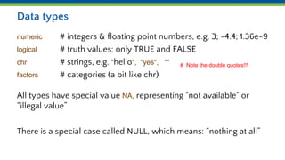
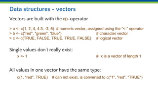
R structures & objects
Day 1 - Introduction to R for Life Sciences
R: a calculator on steroids
The most basic use of R, is that as a calculator:
> 3+2
5
> 5*12
60
But it can do much more
Data types
numeric # integers & floating point numbers, e.g. 3; -4.4; 1.36e-9
logical # truth values: only TRUE and FALSE
chr # strings, e.g. "hello", "yes", ""
factors # categories (a bit like chr)
All types have special value NA, representing "not available" or
“illegal value”
There is a special case called NULL, which means: “nothing at all”
# Note the double quotes!!!
Variables and assignment
Variables contain values. This can also be more than a single item.
Variables are created as soon as you assign a value
Previous value, if any is, overwritten
> mynumber <- 24.3 # mnemonic: 24.3 ‘goes into’ mynumber
> mycharacter <- "foobar" # (also called a ‘value’, even though not numerical)
Data types & variables
Variable names are case-sensitive!
The following variables are all different:
> mynumber <- 24.3
> MyNumber <- 24.3
> my.number <- 24.3 # dot (‘.’) and underscore (‘_’) are often used to make variable names
> my_number <- 24.3 # more readable. They have no special significance
> "foobar" # is a literal value
> foobar # is a variable
Data structures
Vectors
Matrices
Data.frames
Lists
Data structures - vectors
Vectors are built with the c()-operator
> a <- c(1, 2, 4, 4.3, -3, 6) # numeric vector, assigned using the “<-” operator
> b <- c("red", "green", "blue") # character vector
> c <- c(TRUE, FALSE, TRUE, TRUE, FALSE) # logical vector
Single values don’t really exist:
x <- 1 # x is a vector of length 1
All values in one vector have the same type:
c(1, "red", TRUE) # can not exist, is converted to c("1", "red", "TRUE")
Creating vectors
> a <- c(1, 10, 11)
> b <- c(20, 30)
> d <- c(a, 12)
> e <- c(12, a) # note: different from d!
> f <- c(b, d)
> b <- c(b, 40)
> a <- seq(1, 5, 1) # shorthand for this: a <- 1:5
[1] 1 2 3 4 5
> b <- rep(1:3, 2)
[1] 1 2 3 1 2 3
> c <- runif(10) # generate 10 random values
When in doubt, consult the function’s documentation, e.g. ?runif
Convenience functions for creating vectors
Matrices
A matrix is a “vector in the shape of a table”
All items in the matrix are the same data type
Can be built from rows using rbind(), or from columns using cbind(),
or using matrix()
> rbind( 1:3, 11:13)
[,1] [,2] [,3]
[1,] 1 2 3
[2,] 11 12 13
> cbind(11:13, 23:25)
[,1] [,2]
[1,] 11 23
[2,] 12 24
[3,] 13 25
Using the matrix function
> x <- matrix(1:6, nrow=2, byrow=TRUE)
[,1] [,2] [,3]
[1,] 1 2 3
[2,] 4 5 6
Row and column names make life easier!
> x <- matrix(1:6, nrow=2, byrow=TRUE,
dimnames=list( c(“geneA”, “geneB”), c(“delA”, “delB”, “delC”))
delA delB delC
geneA 1 2 3
geneB 4 5 6
Data structures - data.frames
Data.frame: a more general form of a matrix, its columns can be
different type
> id <- c(1, 2, 3, 4)
> color <- c("red", "green", "blue", NA)
> passed <- c(TRUE, TRUE, TRUE, FALSE)
> mydata <- data.frame(id, color, passed)
id color passed
1 1 red TRUE
2 2 green TRUE
3 3 blue TRUE
4 4 <NA> FALSE
Data structures - lists
An ordered collection of "things"
> a <- c(1, 2, 3, 4)
> mylist <- list(name="Patrick", numbers=a, age=38)
$name
[1] "Patrick"
$numbers
[1] 1 2 3 4
$age
[1] 38
Data types - factors
Factors deal with categorical variables
> gender <- factor(c(rep("male", 2), rep("female", 3)))
> gender
[1] male male female female female the actual values
Levels: female male allowed values
> str(gender)
Factor w/ 2 levels "female","male": 2 2 1 1 1
Operations are always element-wise
> a <- 1:3
> b <- 4:6
> a + b
5 7 9
> b^a # ‘raised to power’
4 25 216
> p <- matrix(1:4, ncol=2,
byrow=TRUE)
> q <- cbind(c(10, 10), c(100,100))
> p*q
[,1] [,2]
[1,] 10 200
[2,] 30 400
Auto-recycling of vector content
If you combine vectors of different length, R will automatically
recycle vector content to the longest of the two:
> mynumbers <- c(10.4, 5, 8.4, 3)
> mynumbers2 <- mynumbers + 1
> mynumbers2
11.4, 6, 9.4, 4
What in fact happens is
> mynumbers2 <- mynumbers + c(1, 1, 1, 1)
Useful functions
str() # display the data structure
summary() # display a summary of the data
length() # get the length of a vector or list (data.frame: nrow!)
dim() # get the dimensions of a data.frame or matrix
head() # show the first part of a data structure
You can also explore your data in the Environment window!

Day 1b R structures objects.pptx

  • 1.
    R structures &objects Day 1 - Introduction to R for Life Sciences
  • 2.
    R: a calculatoron steroids The most basic use of R, is that as a calculator: > 3+2 5 > 5*12 60 But it can do much more
  • 3.
    Data types numeric #integers & floating point numbers, e.g. 3; -4.4; 1.36e-9 logical # truth values: only TRUE and FALSE chr # strings, e.g. "hello", "yes", "" factors # categories (a bit like chr) All types have special value NA, representing "not available" or “illegal value” There is a special case called NULL, which means: “nothing at all” # Note the double quotes!!!
  • 4.
    Variables and assignment Variablescontain values. This can also be more than a single item. Variables are created as soon as you assign a value Previous value, if any is, overwritten > mynumber <- 24.3 # mnemonic: 24.3 ‘goes into’ mynumber > mycharacter <- "foobar" # (also called a ‘value’, even though not numerical)
  • 5.
    Data types &variables Variable names are case-sensitive! The following variables are all different: > mynumber <- 24.3 > MyNumber <- 24.3 > my.number <- 24.3 # dot (‘.’) and underscore (‘_’) are often used to make variable names > my_number <- 24.3 # more readable. They have no special significance > "foobar" # is a literal value > foobar # is a variable
  • 6.
  • 7.
    Data structures -vectors Vectors are built with the c()-operator > a <- c(1, 2, 4, 4.3, -3, 6) # numeric vector, assigned using the “<-” operator > b <- c("red", "green", "blue") # character vector > c <- c(TRUE, FALSE, TRUE, TRUE, FALSE) # logical vector Single values don’t really exist: x <- 1 # x is a vector of length 1 All values in one vector have the same type: c(1, "red", TRUE) # can not exist, is converted to c("1", "red", "TRUE")
  • 8.
    Creating vectors > a<- c(1, 10, 11) > b <- c(20, 30) > d <- c(a, 12) > e <- c(12, a) # note: different from d! > f <- c(b, d) > b <- c(b, 40)
  • 9.
    > a <-seq(1, 5, 1) # shorthand for this: a <- 1:5 [1] 1 2 3 4 5 > b <- rep(1:3, 2) [1] 1 2 3 1 2 3 > c <- runif(10) # generate 10 random values When in doubt, consult the function’s documentation, e.g. ?runif Convenience functions for creating vectors
  • 10.
    Matrices A matrix isa “vector in the shape of a table” All items in the matrix are the same data type Can be built from rows using rbind(), or from columns using cbind(), or using matrix() > rbind( 1:3, 11:13) [,1] [,2] [,3] [1,] 1 2 3 [2,] 11 12 13 > cbind(11:13, 23:25) [,1] [,2] [1,] 11 23 [2,] 12 24 [3,] 13 25
  • 11.
    Using the matrixfunction > x <- matrix(1:6, nrow=2, byrow=TRUE) [,1] [,2] [,3] [1,] 1 2 3 [2,] 4 5 6 Row and column names make life easier! > x <- matrix(1:6, nrow=2, byrow=TRUE, dimnames=list( c(“geneA”, “geneB”), c(“delA”, “delB”, “delC”)) delA delB delC geneA 1 2 3 geneB 4 5 6
  • 12.
    Data structures -data.frames Data.frame: a more general form of a matrix, its columns can be different type > id <- c(1, 2, 3, 4) > color <- c("red", "green", "blue", NA) > passed <- c(TRUE, TRUE, TRUE, FALSE) > mydata <- data.frame(id, color, passed) id color passed 1 1 red TRUE 2 2 green TRUE 3 3 blue TRUE 4 4 <NA> FALSE
  • 13.
    Data structures -lists An ordered collection of "things" > a <- c(1, 2, 3, 4) > mylist <- list(name="Patrick", numbers=a, age=38) $name [1] "Patrick" $numbers [1] 1 2 3 4 $age [1] 38
  • 14.
    Data types -factors Factors deal with categorical variables > gender <- factor(c(rep("male", 2), rep("female", 3))) > gender [1] male male female female female the actual values Levels: female male allowed values > str(gender) Factor w/ 2 levels "female","male": 2 2 1 1 1
  • 15.
    Operations are alwayselement-wise > a <- 1:3 > b <- 4:6 > a + b 5 7 9 > b^a # ‘raised to power’ 4 25 216 > p <- matrix(1:4, ncol=2, byrow=TRUE) > q <- cbind(c(10, 10), c(100,100)) > p*q [,1] [,2] [1,] 10 200 [2,] 30 400
  • 16.
    Auto-recycling of vectorcontent If you combine vectors of different length, R will automatically recycle vector content to the longest of the two: > mynumbers <- c(10.4, 5, 8.4, 3) > mynumbers2 <- mynumbers + 1 > mynumbers2 11.4, 6, 9.4, 4 What in fact happens is > mynumbers2 <- mynumbers + c(1, 1, 1, 1)
  • 17.
    Useful functions str() #display the data structure summary() # display a summary of the data length() # get the length of a vector or list (data.frame: nrow!) dim() # get the dimensions of a data.frame or matrix head() # show the first part of a data structure You can also explore your data in the Environment window!