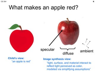
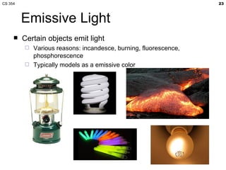
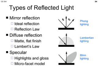
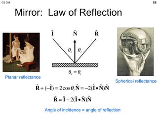
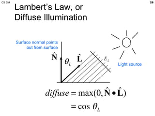
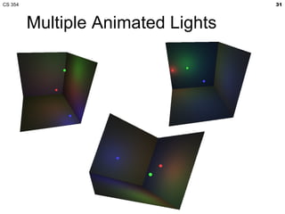
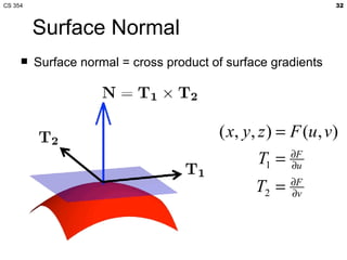
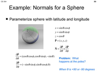
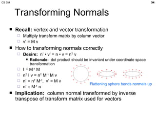
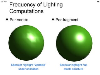
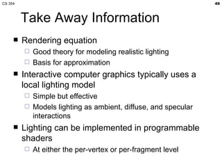
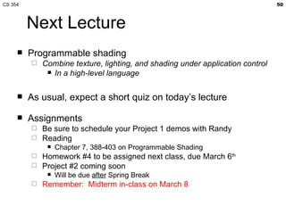
- The lecture covered lighting surfaces in computer graphics, specifically how light interacts with visible surfaces through illumination models like ambient, diffuse, and specular lighting. - Assignments were given including turning in Homework #3, an upcoming Homework #4, and Project #2 on texturing, shading, and lighting due after Spring Break. - A midterm exam was announced for March 8th and office hours were provided for questions.

1. CS 354 Lighting Mark Kilgard University of Texas February 28, 2012

2. Today’s material In-class quiz Lecture topics Lighting surfaces Course work Homework Turn in Homework #3 today Homework #4 to be assigned next class, due March 6th Reading Chapter 7, 388-403 on Programmable Shading Project #2 on texturing, shading, & lighting is coming Will be due after Spring Break Remember: Midterm in-class on March 8

3. My Office Hours Tuesday, before class Painter (PAI) 5.35 8:45 a.m. to 9:15 Thursday, after class ACE 6.302 11:00 a.m. to 12:00

4. Last time, this time Last lecture, we discussed Texture mapping What’s involved in a texel fetch operation? This lecture How do we simulate how light interacts with visible surfaces in computer graphics?

5. Daily Quiz How many texture coordinate components are used to access a cube map? In conventional texture mapping, elements of the texture (texels) store color values. What is stored in the texel values for shadow mapping? If bilinear filtering involves interpolating between 4 texel samples, mipmap bilinear filtering involves filtering how many texels? Multiple choice: The interval between the Texel Selection and Texel Combinations stages of a texture fetch is meant to hide what? a) texture seams b) memory latency c) cache hits d) filtering artifacts e) all of the above On a sheet of paper Write your EID, name, and date Write #1, #2, #3, #4 followed by its answer

6. What makes an apple red? specular diffuse ambient Child’s view: “an apple is red” Image synthesis view: “ light, surface, and material interact to reflect light perceived as color, modeled via simplifying assumptions”

7. Complex Realistic Lighting iray OptiX

8. Why lighting? Convey sense of surface roughness/smoothness Convey sense of material Visual appearance of plastic is different than copper or ebony Realism Emotion Teapots rendered with different material parameters

9. Light Scatters Light strikes A Some scattered Some absorbed Some of scattered light strikes B Some scattered Some absorbed Some of this scattered light strikes A and so on Inherently recursive Massively parallel Points to the ray tracing methodology for rendering

10. Global Lighting Effects translucent surface shadow multiple reflection Common interactive graphics rendering assumption: only model local lighting effects

11. Rendering Equation Theory for light-surface interactions

12. Rendering Equation Parts L o = outgoing light from x in direction ω x = point on a surface ω = normalized outgoing light vector λ = wavelength of light t = time L e = emitted light at x going towards from ω n = surface normal at x

13. Rendering Equation Integral ∫ = integrate over a region Ω = region of a hemisphere Together: “integrate overall the incoming directions for a hemisphere at a point x ” ωˊ = normalized outgoing light vector L i = incoming light at x coming from ωˊ n = surface normal at x (- ωˊ • n ) = cosine of angle between incoming light and surface normal d ωˊ = differential of incoming angle

14. Bidirectional Reflectance Distribution Function Ratio of differential outgoing (reflected) radiance to differential incoming irradiance Physically based BRDF properties Must be non-negative Must be reciprocal Swap incoming & relected directions generates same ratio Conserves energy Integrating over entire hemisphere must be ≤ 1 L = radiance E = irradiance

15. Cosine Weighting for Irradiance At shallow angles, incoming light spreads over a wider area of the surface Thus spreading the energy Thus dimming the received light

16. Measuring BRDFs Empirically Gonioreflectometer is device to measure BRDFs

17. Rendering Equation Interpretation Recursive equation Limitations Treats wavelengths all independent Treats time in Newtonian way Ignores volumetric and subsurface scattering More complex models can incorporate these aspects of light Impractical for actual computer graphics rendering outgoing light “sums up” all incoming light for all surfaces

18. Light Sources Real lights have “emissive regions” Simplifying assumption treats lights as points Model area lights source as “lots of points” Lights have color and attenuation Fall-off, spotlight, and shadow attenuation

19. Area Light Source Modeled as Many Points 12 point light sources model an area light

20. Light Attenuation Energy of light in watts But energy received over a distance surface falls off with the inverse square of the distance from the light Steradian (st) is measure of solid angle

21. Simple Light Source Types Positional (point) light sources (x,y,z,1) Directional (infinite) light sources Represented with homogeneous corodinates (x,y,z,0) Spot light Directional lighting Often a cone or cone with fall-off function Linear light sources Ambient light Useful as an error term Directional light operates as if at infinity Rays are essentially parallel—sun would be such a light

22. Surface Types Smooth surfaces reflect like mirrors Rough surfaces scatter light Real surfaces act as mixture of both Smooth reflective surface Rough diffuse surface

23. Emissive Light Certain objects emit light Various reasons: incandesce, burning, fluorescence, phosphorescence Typically models as a emissive color

24. Types of Reflected Light Mirror reflection Ideal reflection Reflection Law Diffuse reflection Matte, flat finish Lambert’s Law Specular Highlights and gloss Micro-facet model Phong lighting Lambertian lighting Blinn lighting

25. Mirror: Law of Reflection Angle of incidence = angle of reflection Planar reflectance Spherical reflectance

26. Lambert’s Law, or Diffuse Illumination Surface normal points out from surface Light source

27. Micro-facet Specular Think of the surface as have a statistical distribution of facet orientations OpenGL’s fixed-function specular model

28. Shininess Modeled as exponential fall-off function Larger shininess exponent values means a tighter specular highlight Complement of shininess is roughness Exponential fall-off also use to model Spotlight attenuation Fog effects

29. Combining Lighting Contributions Contributions can be summed Since RGB color components are additive Illumination color modulated by material color Ambient Diffuse Specular Result

30. Summing Multiple Lights For each light source and each color component, the Blinn or Phong model can be written (without the distance terms) as I = k d l d l · n + k s I s ( v · r )  + k a I a I = k d l d l · n + k s I s ( h · n )  + k a I a For each color component, we add contributions from all sources Blinn Phong

31. Multiple Animated Lights

32. Surface Normal Surface normal = cross product of surface gradients

33. Example: Normals for a Sphere Parameterize sphere with latitude and longitude Problem: What happens at the poles? When θ is +90 or -90 degrees

34. Transforming Normals Recall: vertex and vector transformation Multiply transform matrix by column vector v’ = M v How to transforming normals correctly Desire: n’ • v’ = n • v = n T v Rationale: dot product should be invariant under coordinate space transformation I = M -1 M n T I v = n T M -1 M v n’ = n T M -1 , v’ = M v n’ = M -T n Implication: column normal transformed by inverse transpose of transform matrix used for vectors Flattening sphere bends normals up

35. Frequency of Lighting Computations Per-vertex Per-fragment Specular highlight “wobbles” under animation Specular highlight has stable structure

36. Fixed-function OpenGL Per-vertex Lighting OpenGL API includes lighting model Operates at the per-vertex level Implements a Blinn-Phong lighting model Example usage glEnable ( GL_LIGHTING ); glEnable ( GL_LIGHT0 ); glLightfv ( GL_LIGHT0 , GL_POSITION , position); glLightfv ( GL_LIGHT0 , GL_DIFFUSE , diffuse); glLightfv ( GL_LIGHT0 , GL_SPECULAR , specular); Relies on Per-vertex normal value sent with glNormal3f And per-vertex material properties sent with glMaterialfv

37. OpenGL Light Parameters Per-light state set with glLightfv command Scalar float Scalar float Scalar float Angle in degrees Non-negative scalar exponent Direction vector, 3 floats Homogeneous position, 4 floats RGBA, 4 floats RGBA, 4 floats RGBA, 4 floats Type 0 Inverse quadratic attenuation GL_QUADRATIC_ATTENUATION 0 Inverse linear attenuation GL_LINEAR_ATTENUATION 1 Light attenuation inverse constant GL_CONSTANT_ATTENUATION 180, uniform distribution Angle of spot light cut off GL_SPOT_CUTOFF 0 Spot light exponential fall-off GL_SPOT_EXPONENT (0,0,-1) Spot light direction GL_SPOT_DIRECTION (0,0,1,0), +Z axis direction Light location GL_POSITION (1,1,1,1) for light 0, (0,0,0,1) for other lights Specular light color GL_SPECULAR (1,1,1,1) for light 0, (0,0,0,1) for other lights Diffuse light color GL_DIFFUSE (0,0,0,1) Ambient light color GL_AMBIENT Initial Value Meaning Token Name

38. OpenGL Material Parameters Per-light state set with glLightfv command Surface has GL_FRONT and GL_BACK versions of these materials For two-sided lighting, depending on how polygon faces Scalar float RGBA, 4 floats RGBA, 4 floats RGBA, 4 floats RGBA, 4 floats Type 0 Specular exponent of material GL_SHININESS (0, 0, 0, 1) Emissive material color GL_EMISSION (0, 0, 0, 1) Specular material color GL_SPECULAR (0.8, 0.8, 0.8, 1) Diffuse material color GL_DIFFUSE (0.2, 0.2, 0.2, 1) Ambient material color GL_AMBIENT Initial Value Meaning Token Name

39. OpenGL Fixed-function Lighting Equation emissive global ambient for each light source surface result color per-light ambient diffuse specular diffuse squashes specular

40. OpenGL Lighting Equation Terms half-angle distance attenuation spotlight attenuation infinite viewer assumption local viewer assumption inverse square fall-off

41. Displacement and Bump Mapping Use surface offsets stored in texture Perturb or displace the surface Shade on the resulting surface normals

42. Normal Mapping Bump mapping via a normal map texture Instead of a height field The normal map is generated from the height field  + diffuse decal specular =

43. Combination of Normal Map Lighting + Texturing   ) + ( ( ) = Diffuse Gloss Specular Decal Final result!

44. Environment Mapping as Omni-directional Lighting Access texture by surface reflection vector

45. Other Fancy Lighting Effects Caustic patterns Light is “focused” as it refracts through interfaces Diffraction Small slits act as a diffraction grating, separating wavelengths

46. Subsurface Scattering Light bounces around within an object Translucency

47. Paths of Scattered Photons Trace photons statistically as they bounce and eventually exit the material

48. Accurate Skin Needs to Model Subsurface Scattering Skin with subsurface scattering Looks natural Without Looks lifeless Credit: Stephen Stahlberg

49. Take Away Information Rendering equation Good theory for modeling realistic lighting Basis for approximation Interactive computer graphics typically uses a local lighting model Simple but effective Models lighting as ambient, diffuse, and specular interactions Lighting can be implemented in programmable shaders At either the per-vertex or per-fragment level

50. Next Lecture Programmable shading Combine texture, lighting, and shading under application control In a high-level language As usual, expect a short quiz on today’s lecture Assignments Be sure to schedule your Project 1 demos with Randy Reading Chapter 7, 388-403 on Programmable Shading Homework #4 to be assigned next class, due March 6 th Project #2 coming soon Will be due after Spring Break Remember: Midterm in-class on March 8

51. Credits and Appreciation Some images from Dr. Pat Hanrahan, Stanford University Ed Angel & David Shriner, textbook Stephen Stahlberg Christian Miller, UT CS