Download as PDF, PPTX
![Example
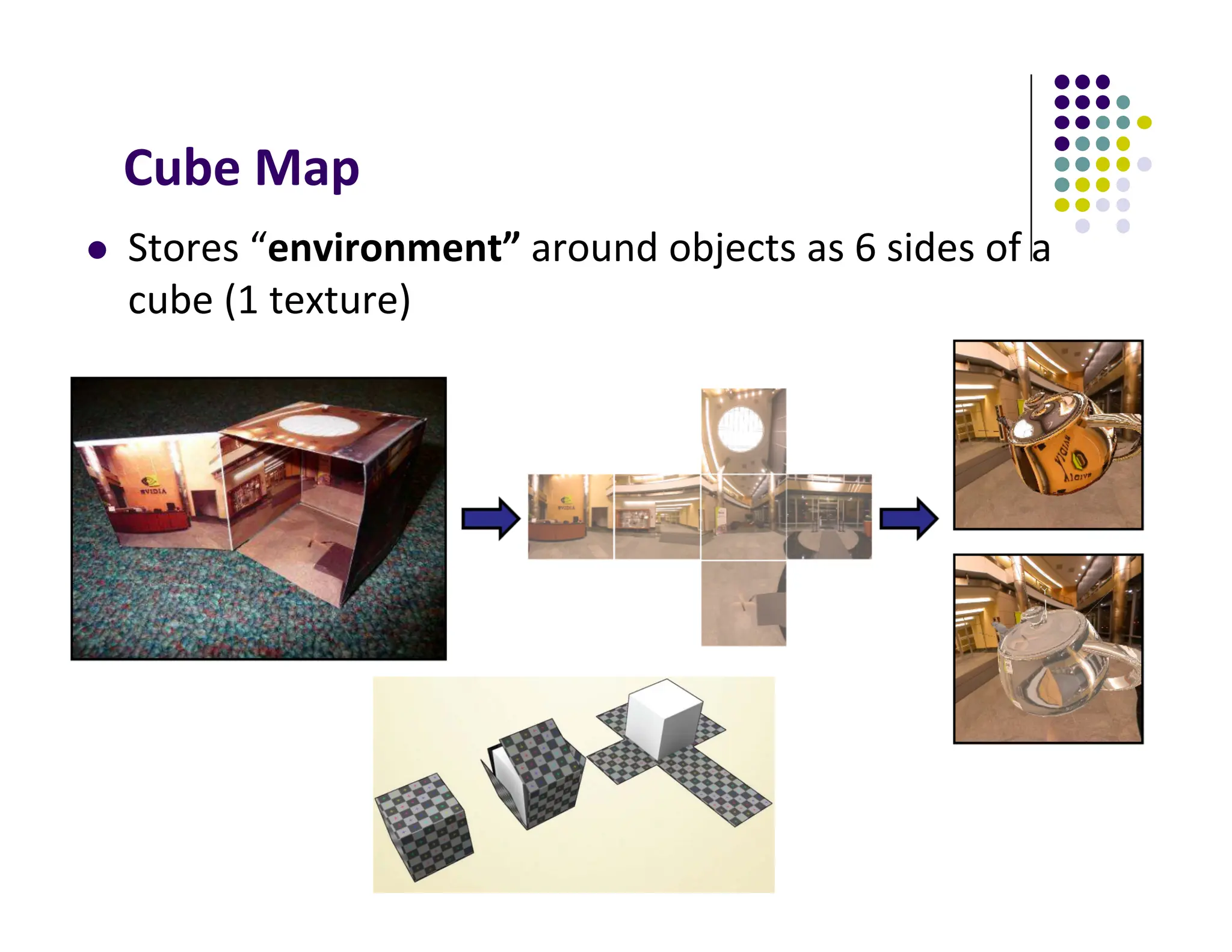
R = (‐4, 3, ‐1)
Same as R = (‐1, 0.75, ‐0.25)
Use face x = ‐1 and y = 0.75, z = ‐0.25
Not quite right since cube defined by x, y, z = ± 1
rather than [0, 1] range needed for texture
coordinates
Remap by s = ½ + ½ y, t = ½ + ½ z
Hence, s =0.875, t = 0.375](https://image.slidesharecdn.com/lecture09p1-250120084342-216af9c6/75/reflective-bump-environment-mappings-pdf-10-2048.jpg)
![Cube Map Example (init)
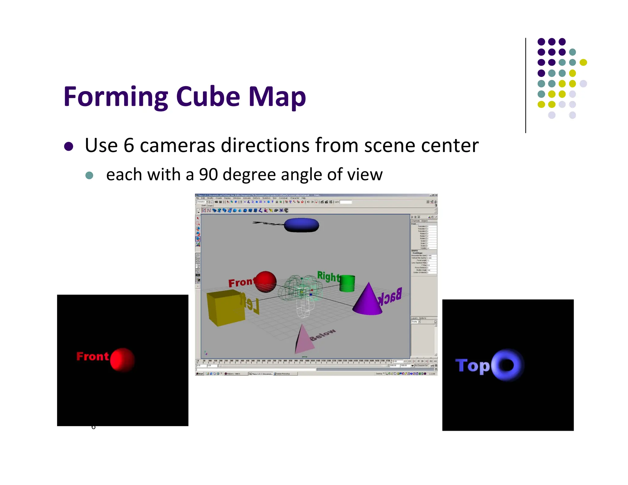
// colors for sides of cube
GLubyte red[3] = {255, 0, 0};
GLubyte green[3] = {0, 255, 0};
GLubyte blue[3] = {0, 0, 255};
GLubyte cyan[3] = {0, 255, 255};
GLubyte magenta[3] = {255, 0, 255};
GLubyte yellow[3] = {255, 255, 0};
glEnable(GL_TEXTURE_CUBE_MAP);
// Create texture object
glGenTextures(1, tex);
glActiveTexture(GL_TEXTURE1);
glBindTexture(GL_TEXTURE_CUBE_MAP, tex[0]);
You can also just load
6 pictures of environment](https://image.slidesharecdn.com/lecture09p1-250120084342-216af9c6/75/reflective-bump-environment-mappings-pdf-12-2048.jpg)
![Cube Map (init III)
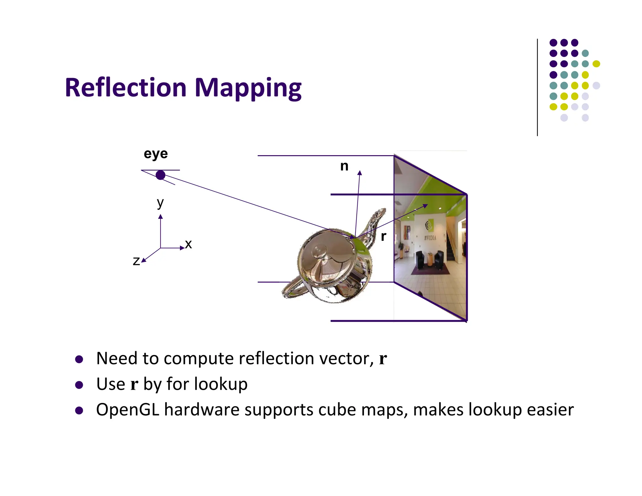
GLuint texMapLocation;
GLuint tex[1];
texMapLocation = glGetUniformLocation(program, "texMap");
glUniform1i(texMapLocation, tex[0]);
Connect texture map (tex[0])
to variable texMap in fragment shader
(texture mapping done in frag shader)](https://image.slidesharecdn.com/lecture09p1-250120084342-216af9c6/75/reflective-bump-environment-mappings-pdf-14-2048.jpg)
![Adding Normals
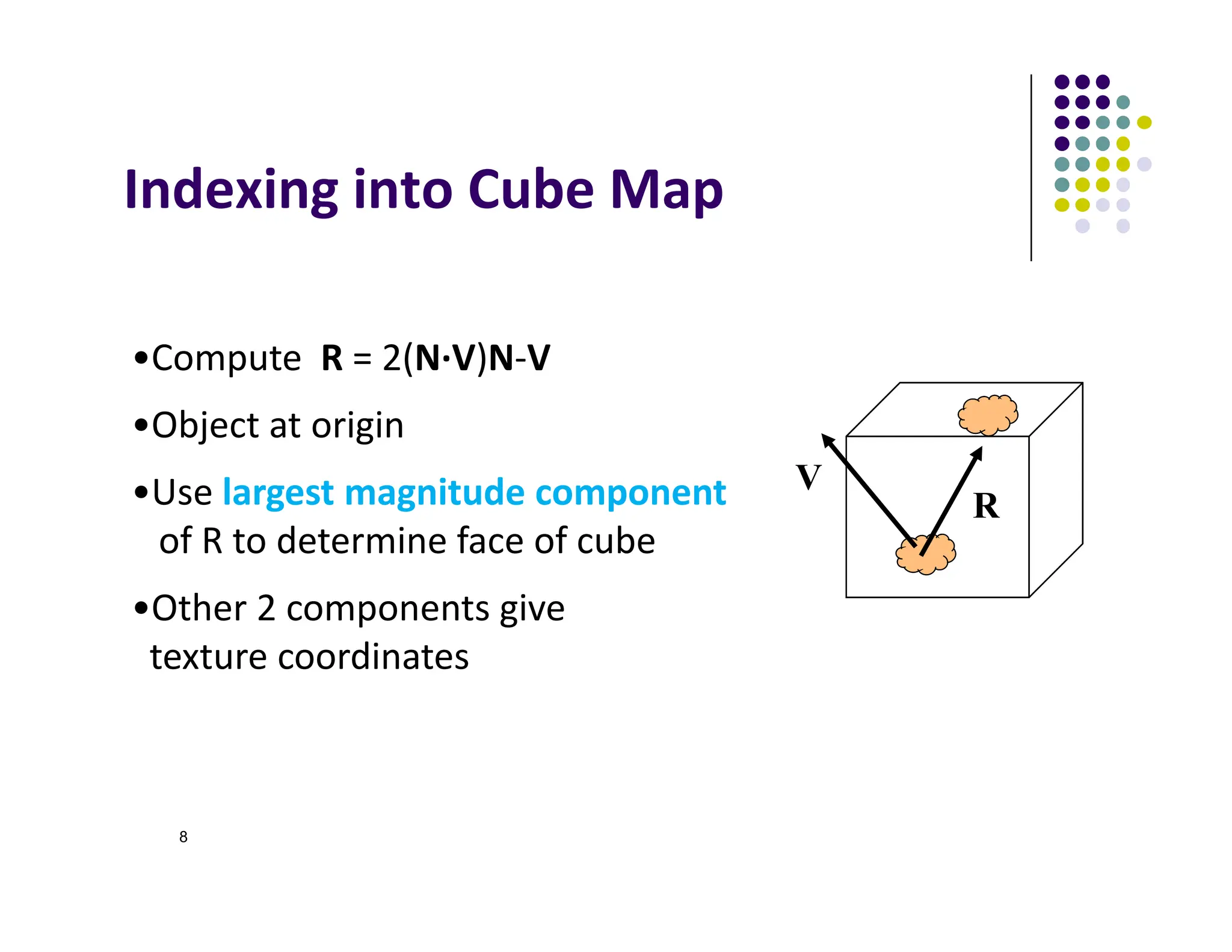
void quad(int a, int b, int c, int d)
{
static int i =0;
normal = normalize(cross(vertices[b] - vertices[a],
vertices[c] - vertices[b]));
normals[i] = normal;
points[i] = vertices[a];
i++;
// rest of data](https://image.slidesharecdn.com/lecture09p1-250120084342-216af9c6/75/reflective-bump-environment-mappings-pdf-15-2048.jpg)
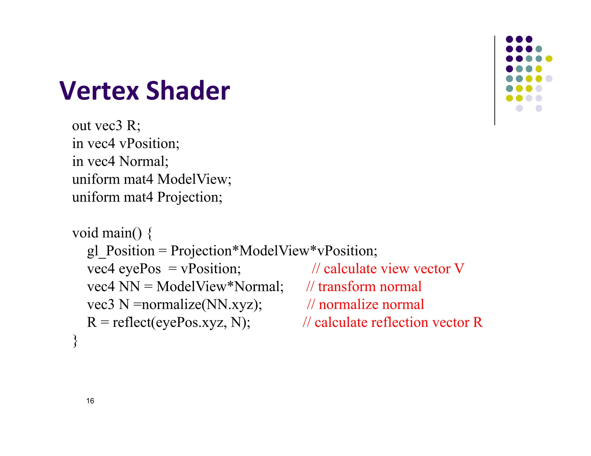

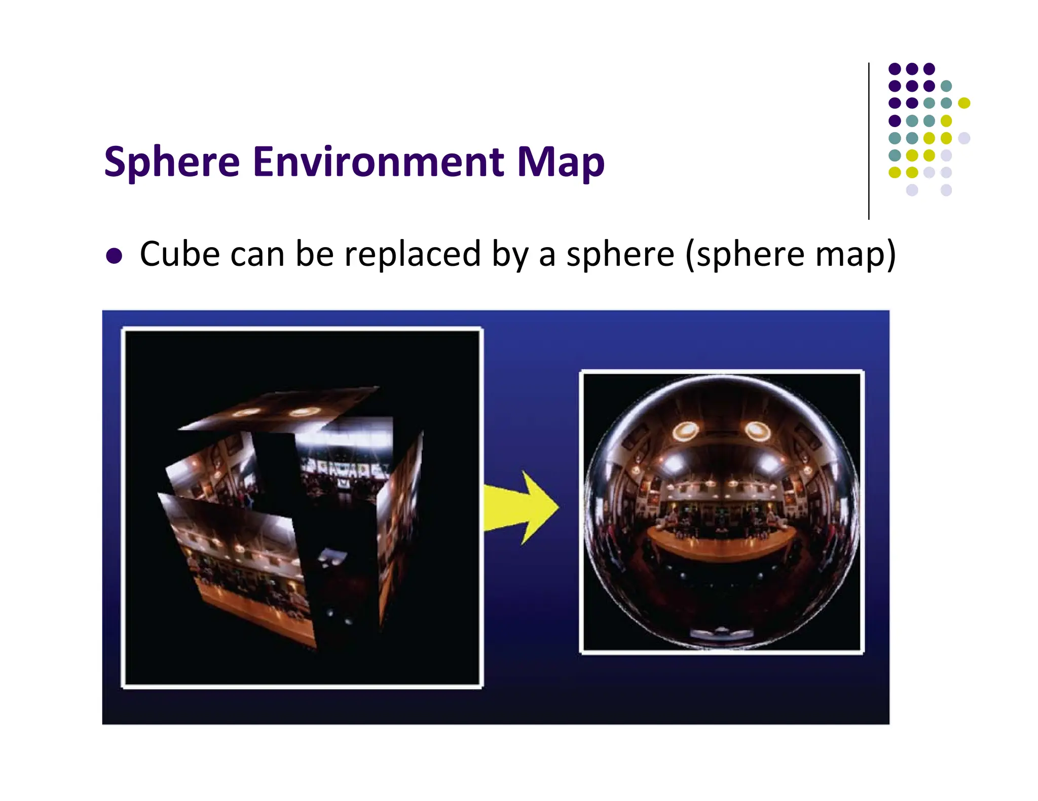


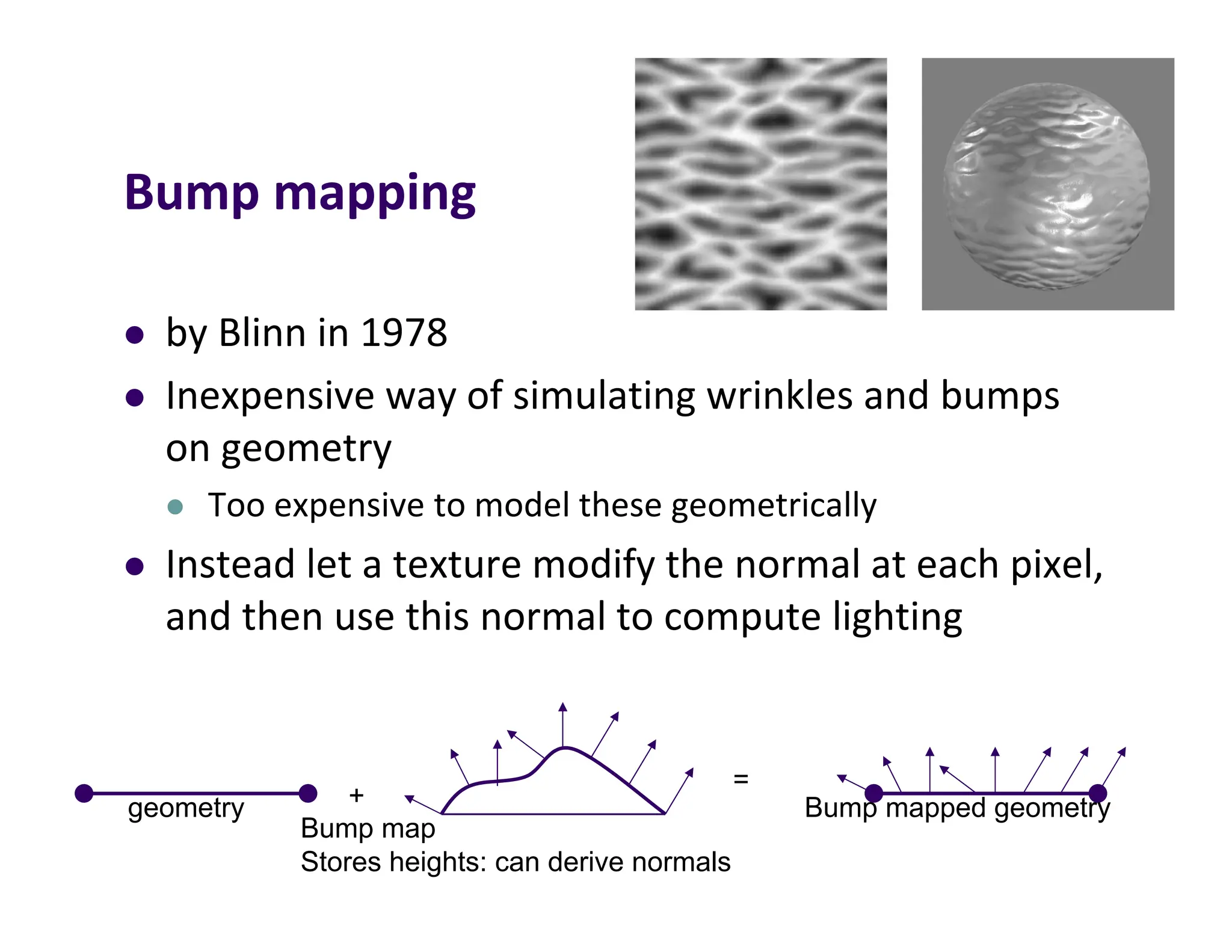
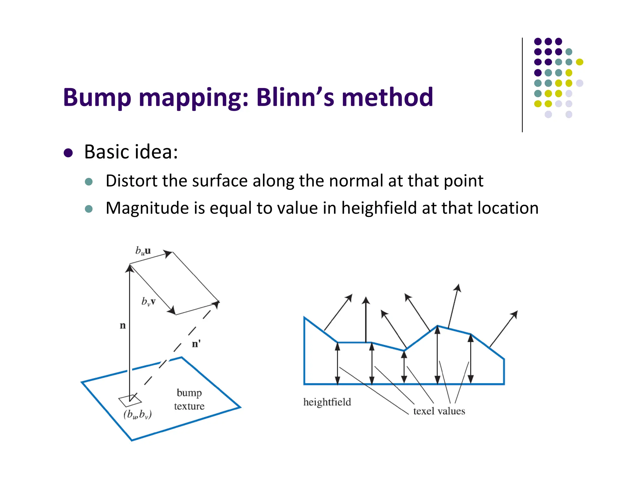
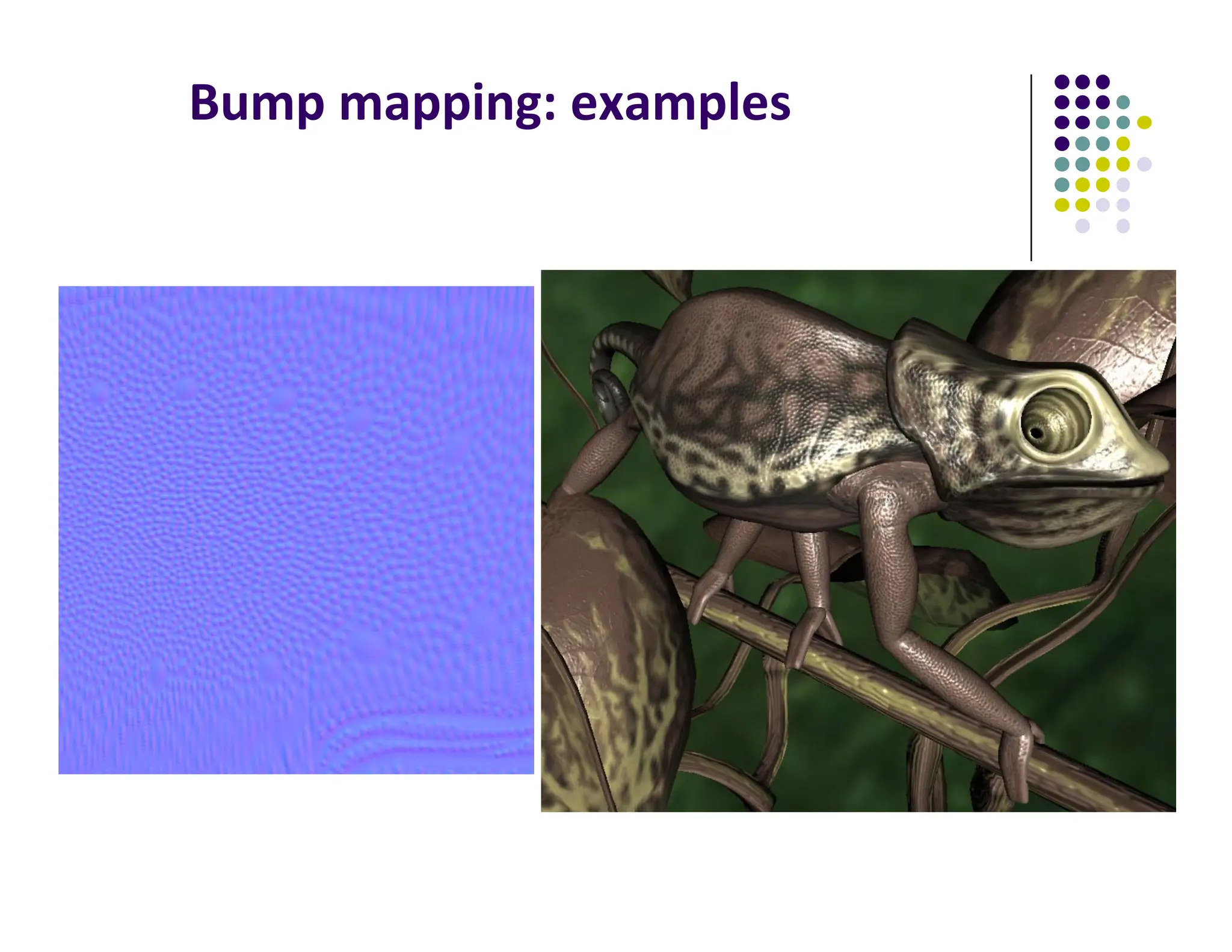
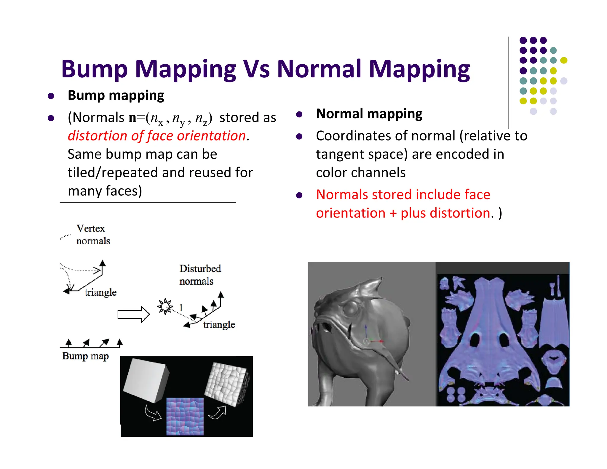
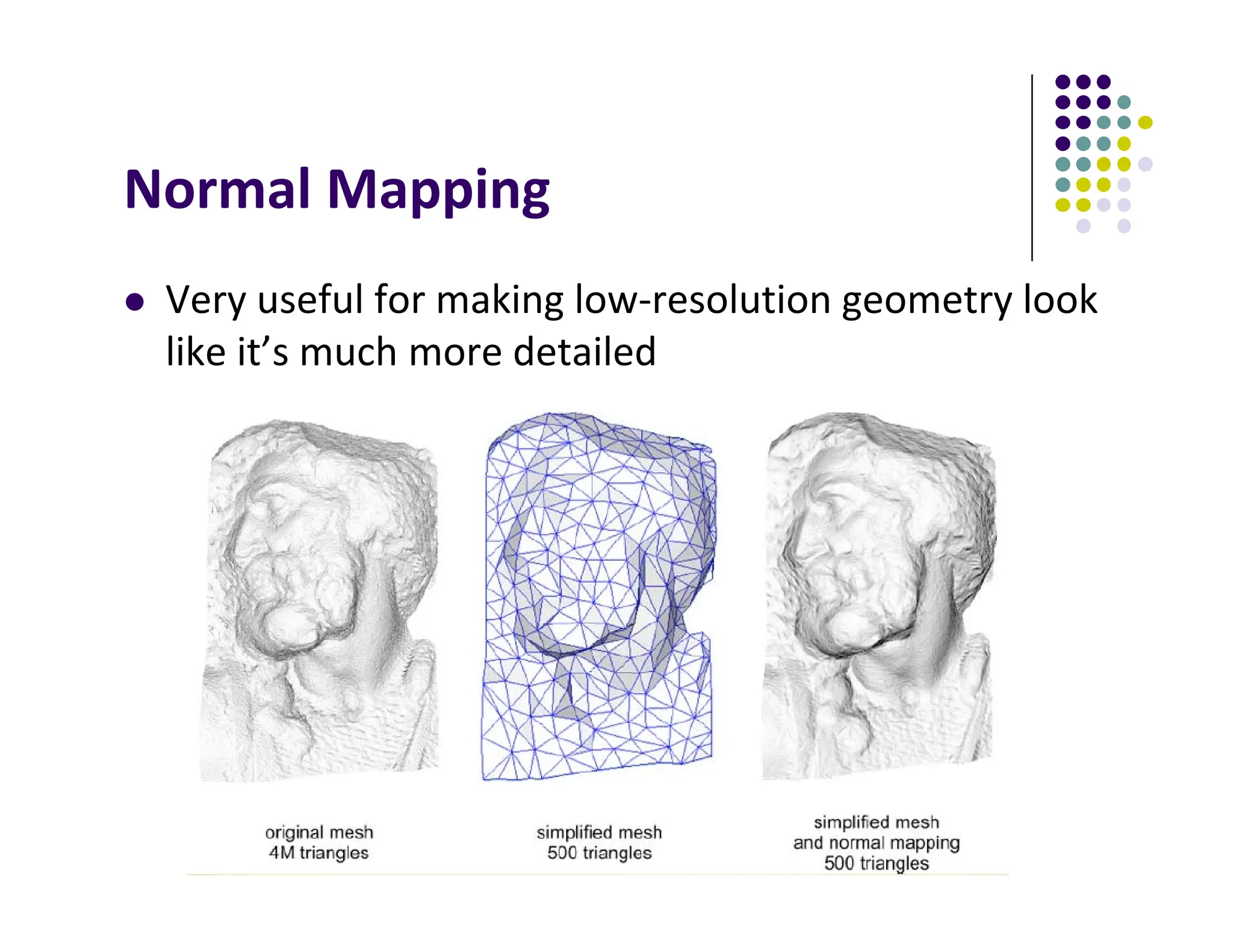

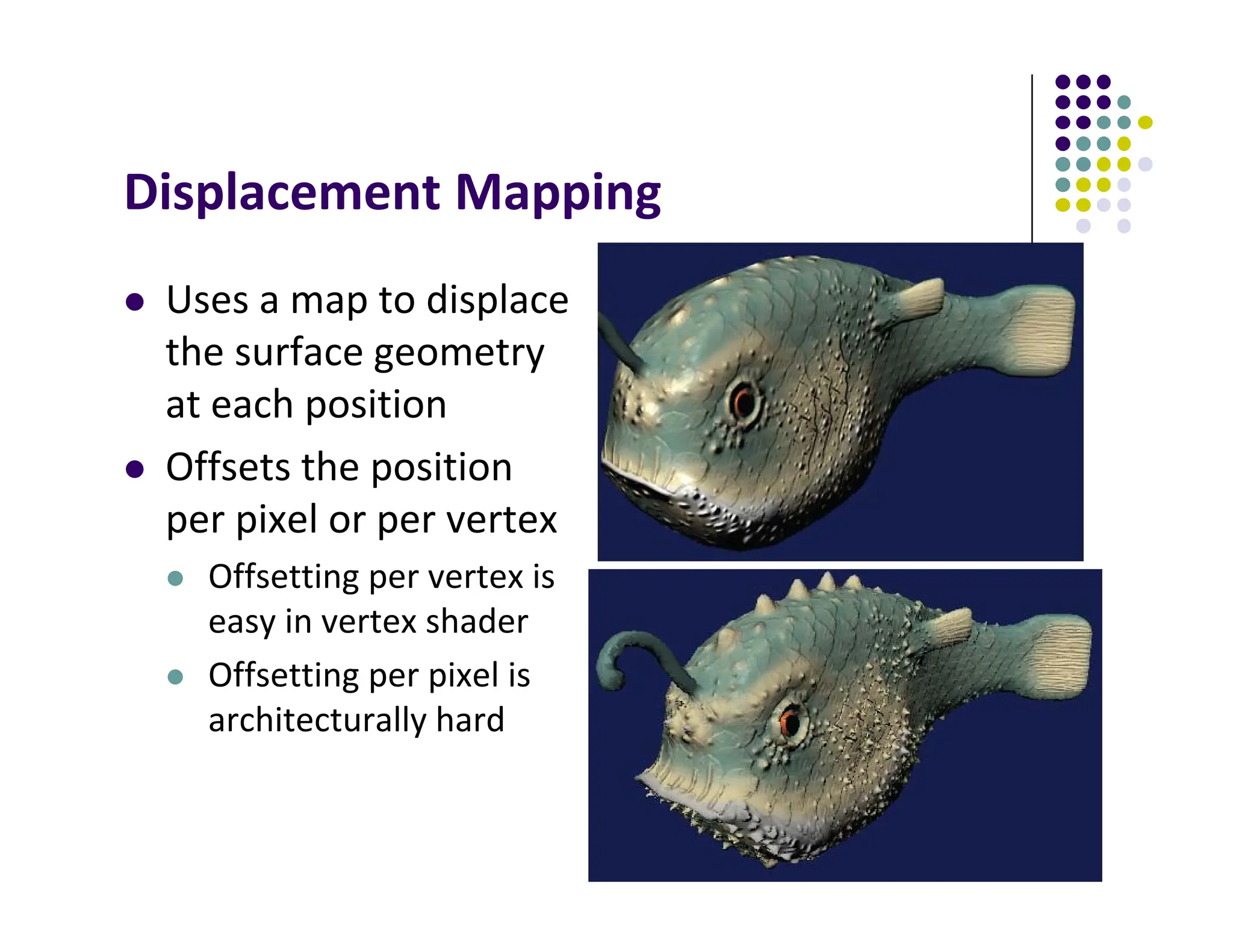
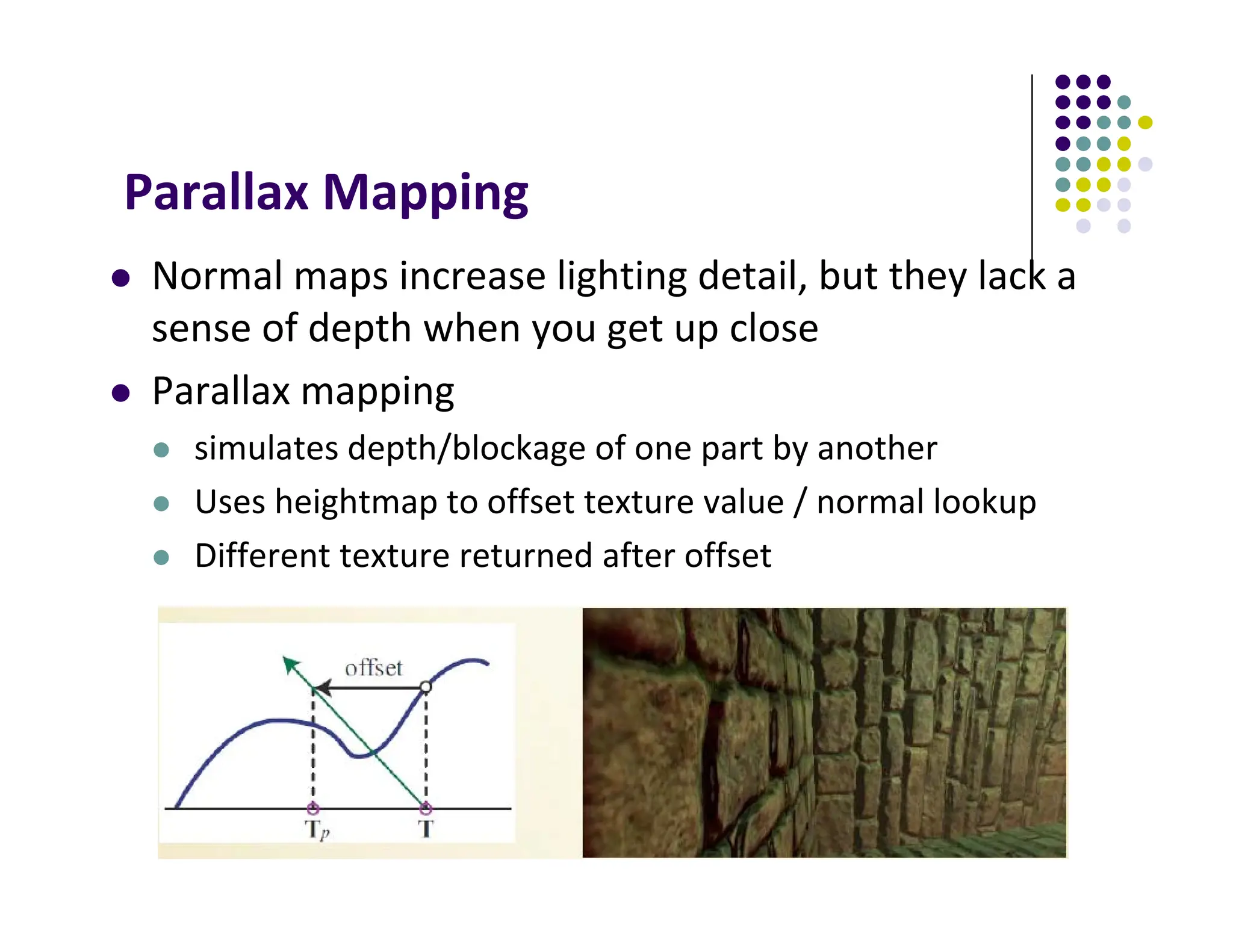
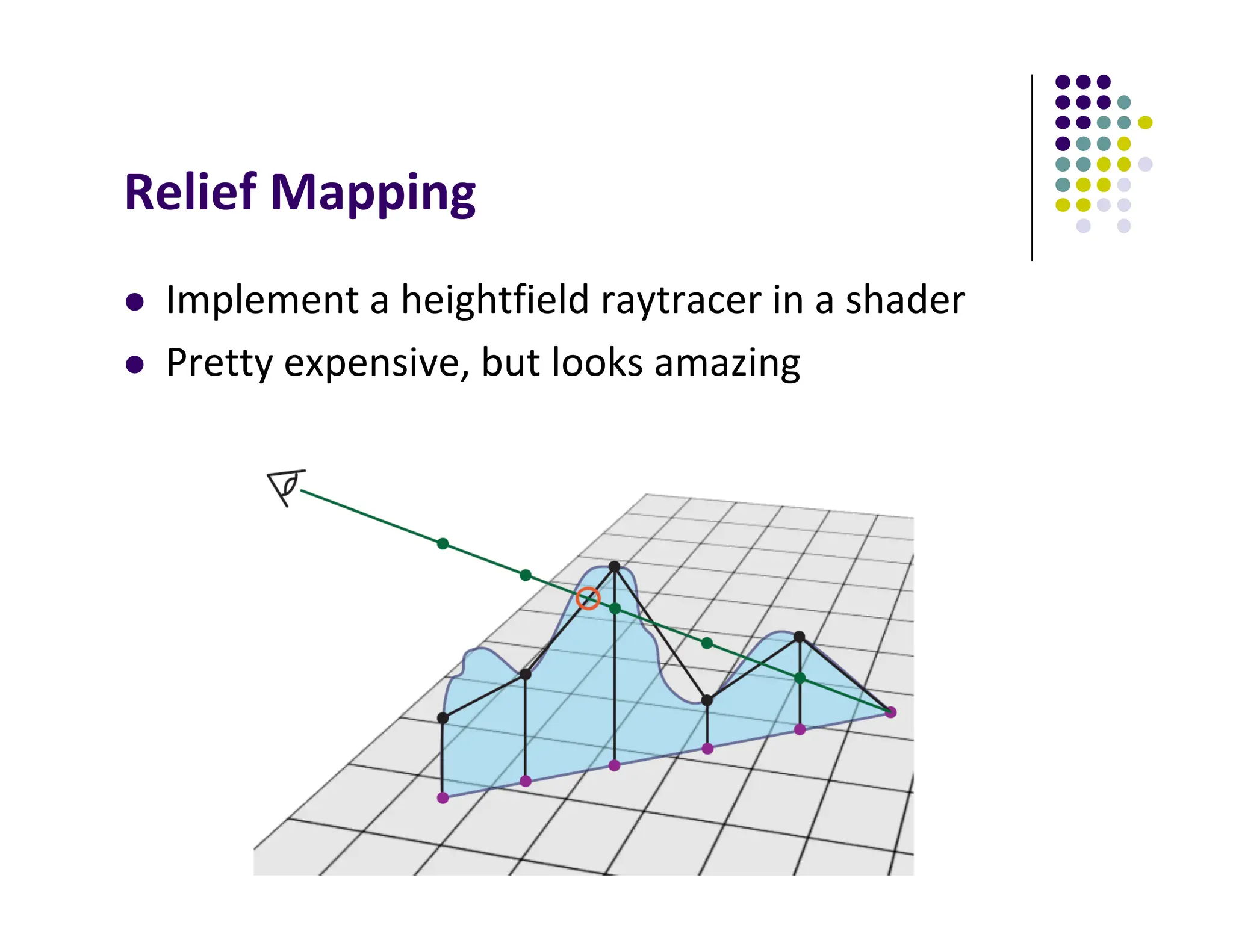
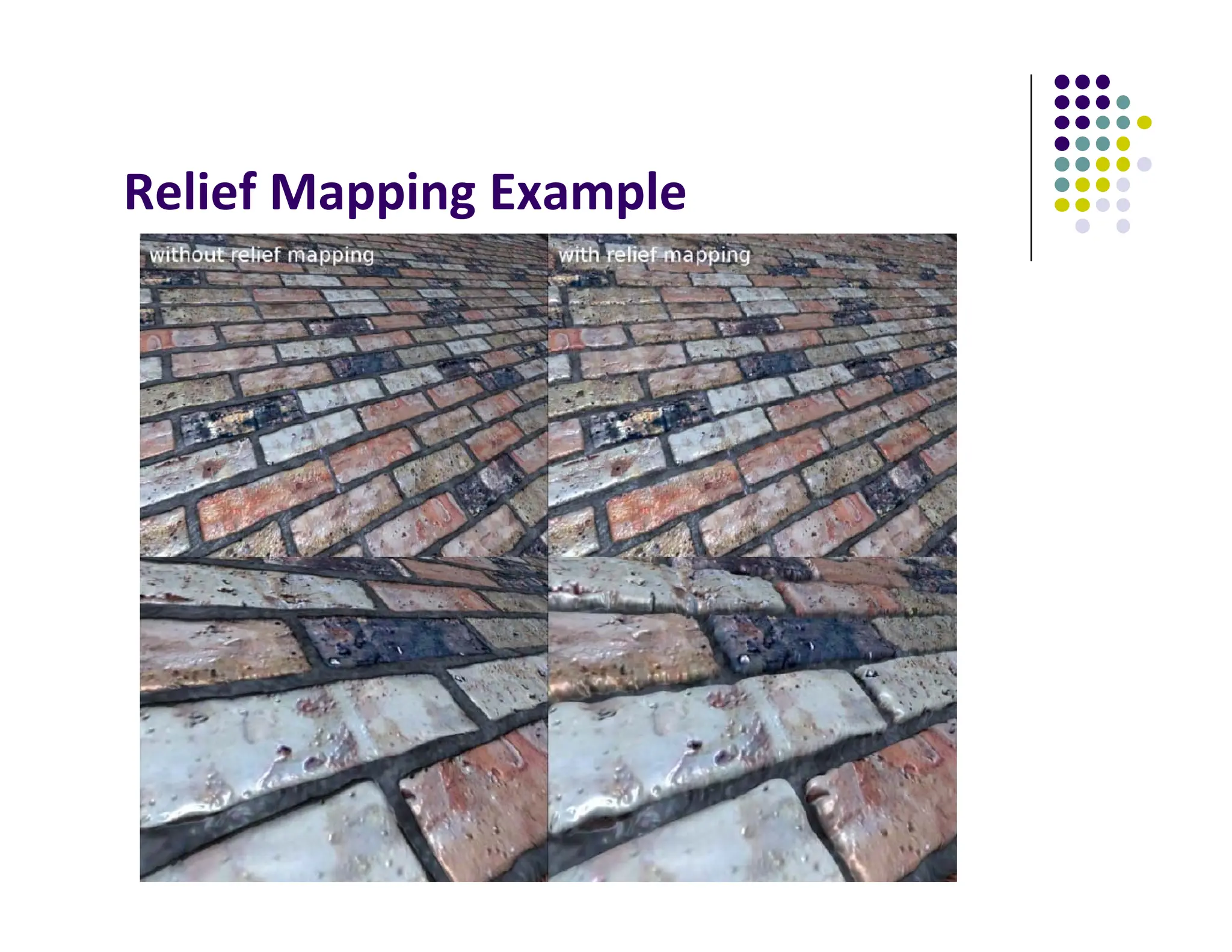


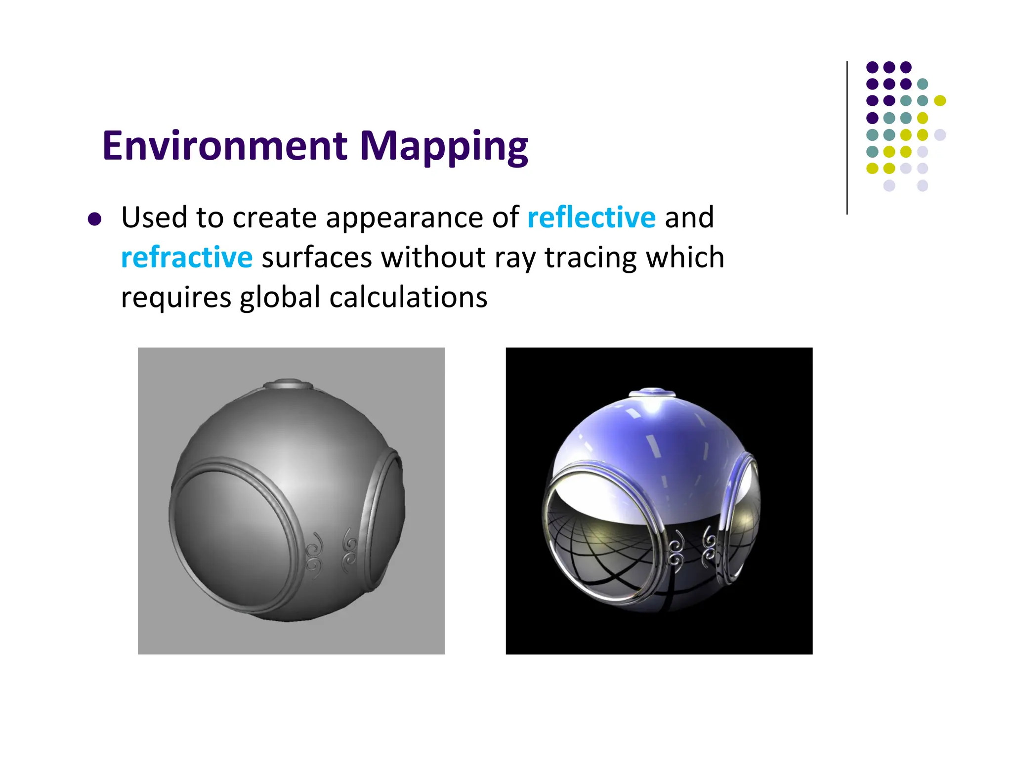
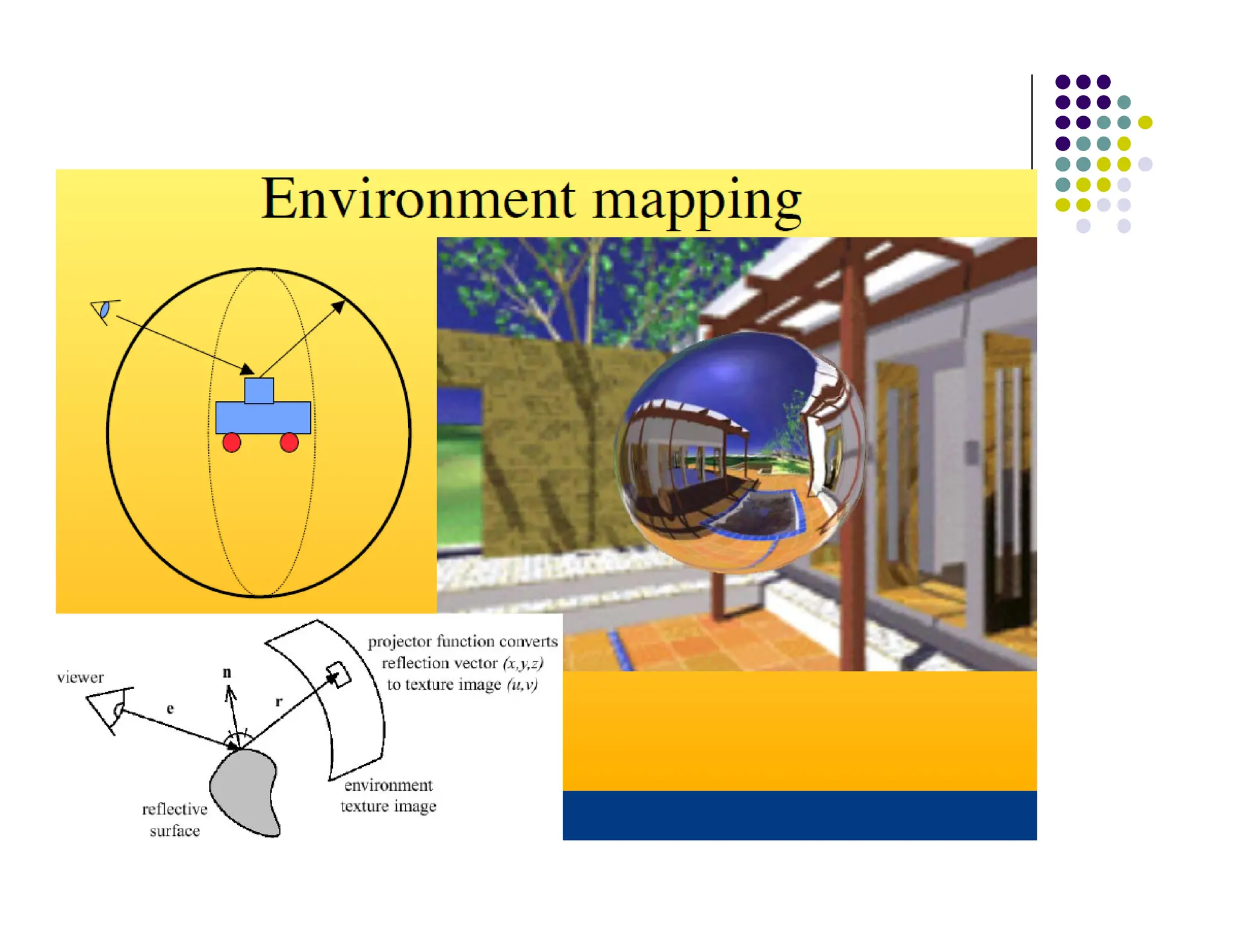
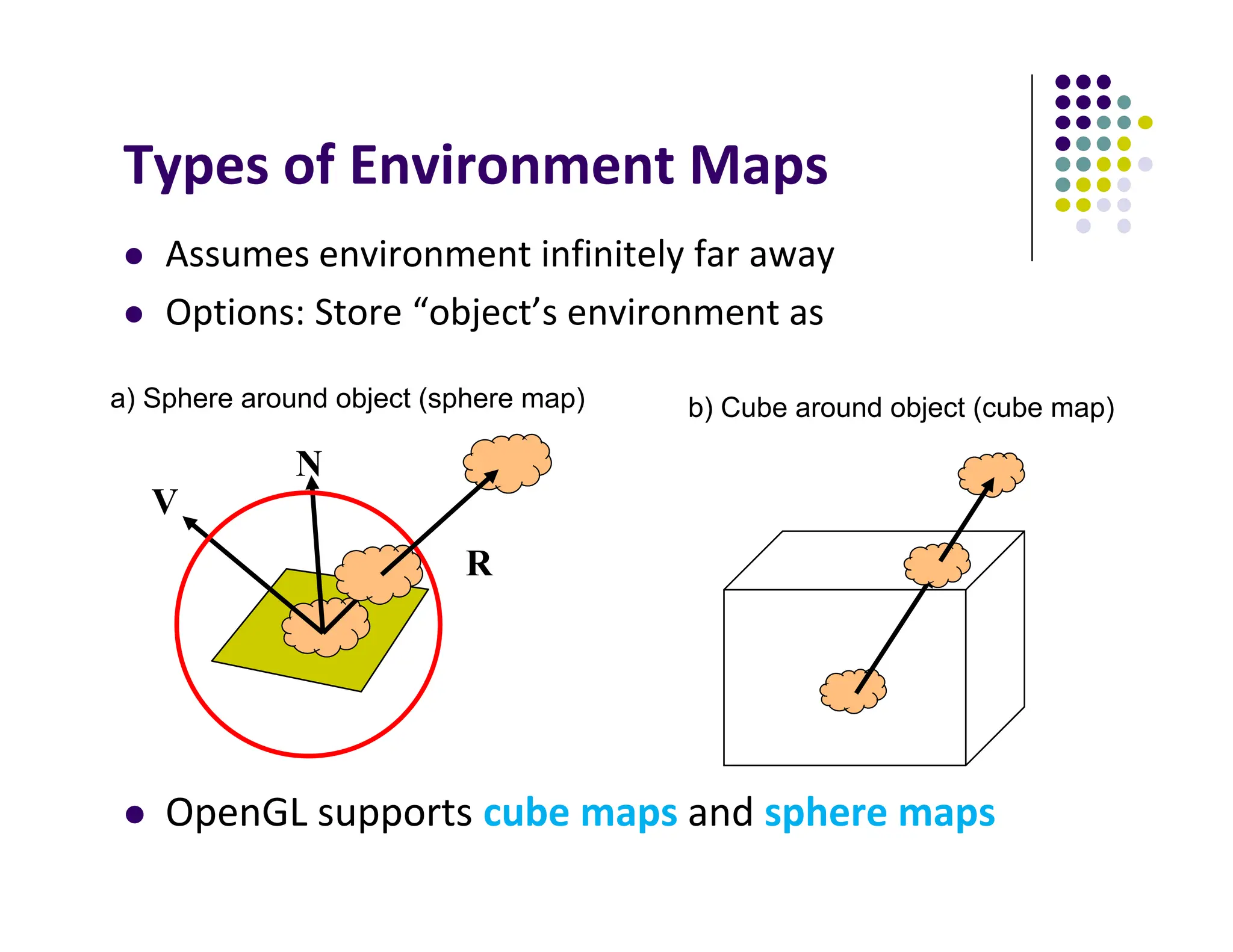
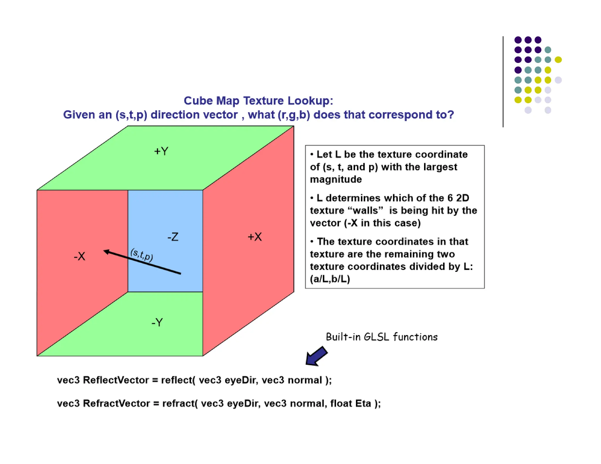
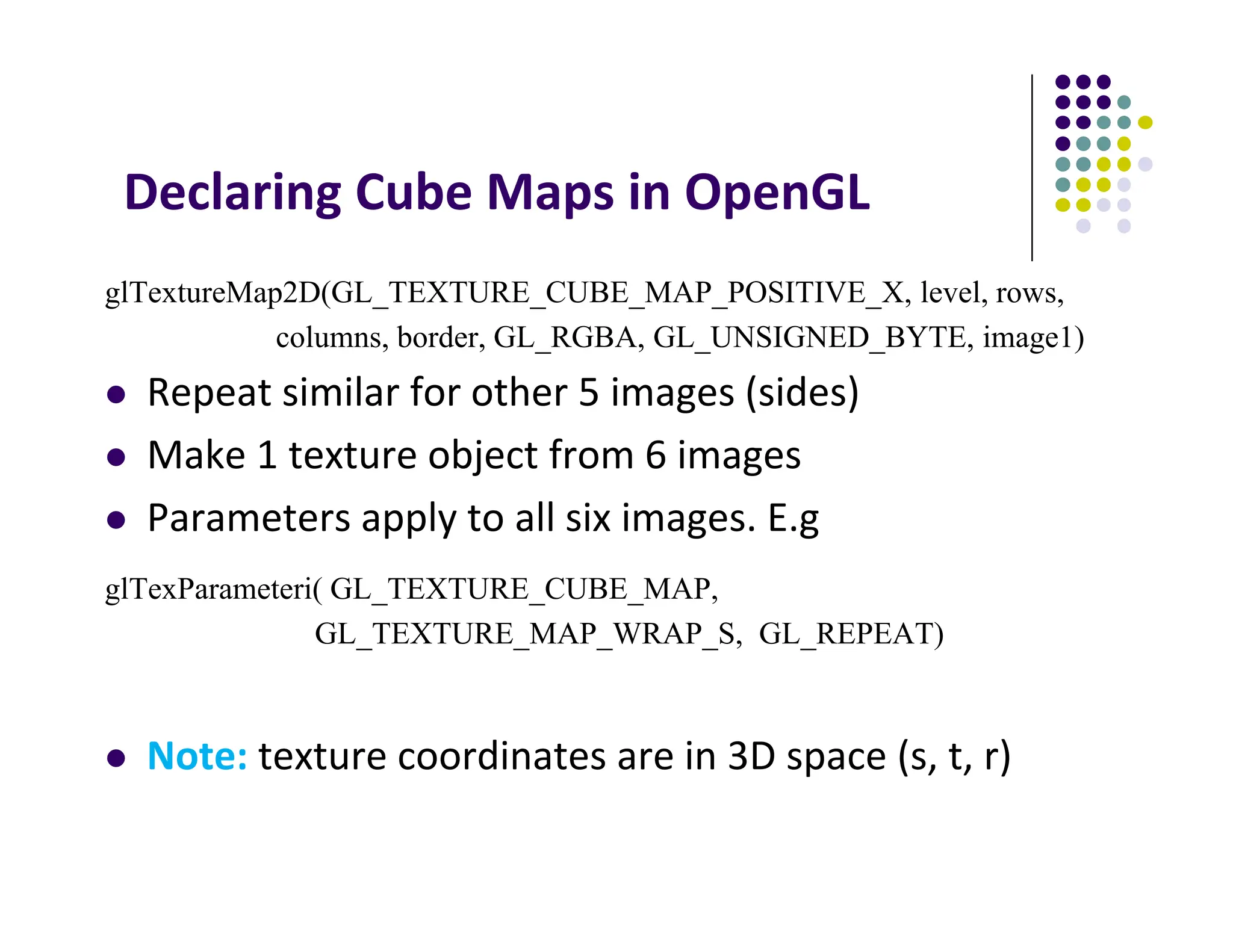
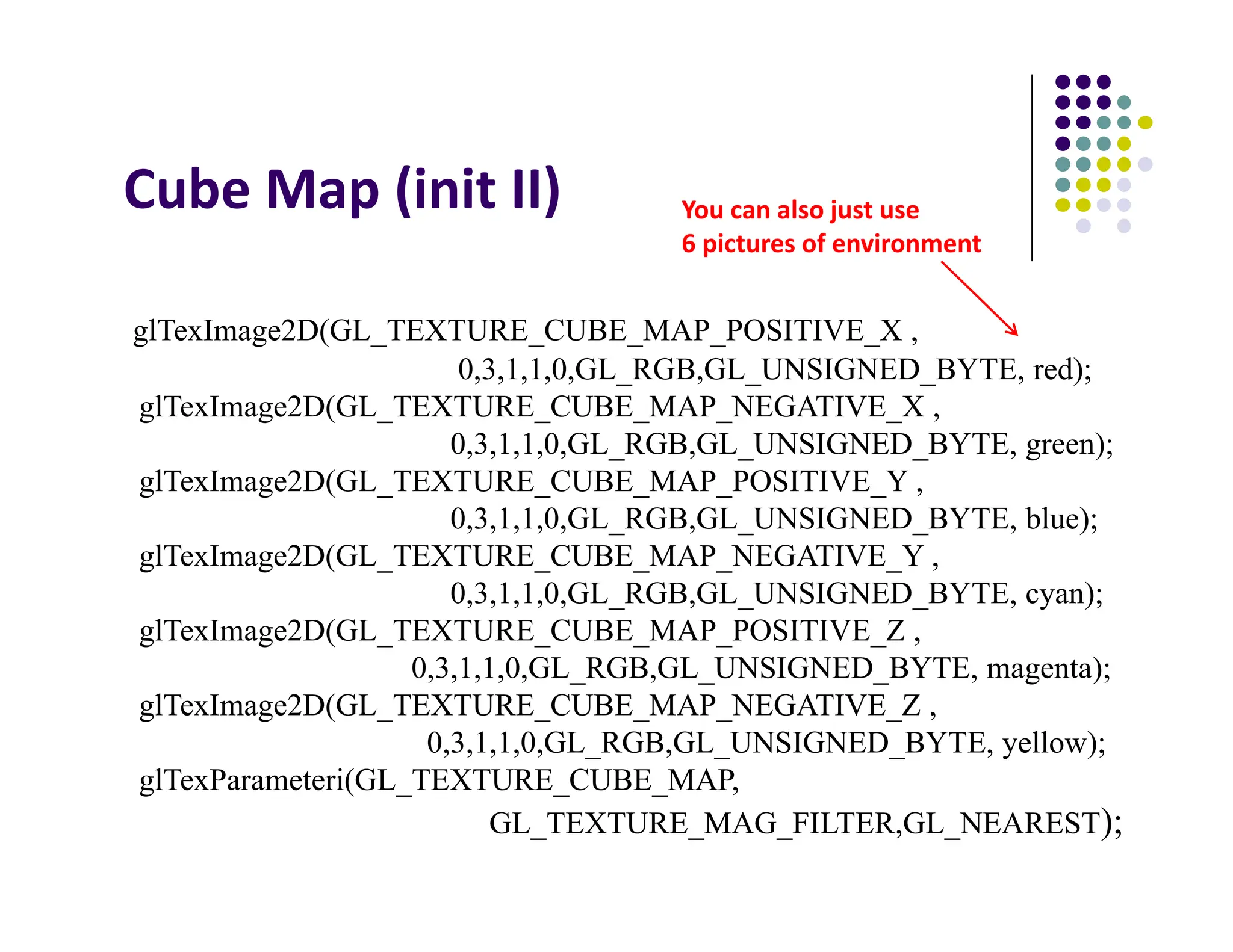
The document discusses environment mapping techniques in computer graphics, focusing on creating reflections and refractions without ray tracing by using cube and sphere maps. It explains how these maps are defined, how to calculate reflection and refraction vectors, and the implementation of these techniques in OpenGL. Additionally, it covers various texturing methods such as bump mapping, normal mapping, displacement mapping, and parallax mapping to enhance realism in 3D graphics.