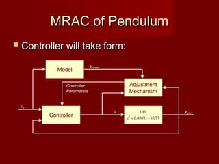
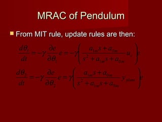
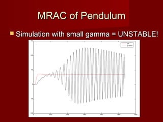
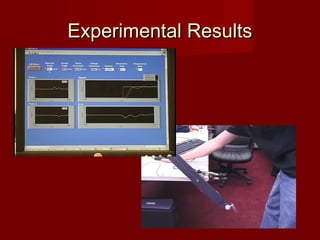
Model ReferenceModel Reference
Adaptive ControlAdaptive Control
Survey of Control Systems (MEM 800)Survey of Control Systems (MEM 800)
Presented byPresented by
Keith SevcikKeith Sevcik
ConceptConcept
 Design controller to drive plant response to mimic idealDesign controller to drive plant response to mimic ideal
response (error = yresponse (error = yplantplant-y-ymodelmodel => 0)=> 0)
 Designer chooses: reference model, controller structure,Designer chooses: reference model, controller structure,
and tuning gains for adjustment mechanismand tuning gains for adjustment mechanism
Controller
Model
Adjustment
Mechanism
Plant
Controller
Parameters
ymodel
u yplant
uc
MIT RuleMIT Rule
 Tracking error:Tracking error:
 Form cost function:Form cost function:
 Update rule:Update rule:
– Change in is proportional to negative gradient ofChange in is proportional to negative gradient of
modelplant yye −=
)(
2
1
)( 2
θθ eJ =
δθ
δ
γ
δθ
δ
γ
θ e
e
J
dt
d
−=−=
θ J
sensitivity
derivative
MIT RuleMIT Rule
 Can chose different cost functionsCan chose different cost functions
 EX:EX:
 From cost function and MIT rule, control law can beFrom cost function and MIT rule, control law can be
formedformed





<−
=
>
=
−=
=
0,1
0,0
0,1
)(where
)(
)()(
e
e
e
esign
esign
e
dt
d
eJ
δθ
δ
γ
θ
θθ
MIT RuleMIT Rule
 EX: Adaptation of feedforward gainEX: Adaptation of feedforward gain
Adjustment Mechanism
ymodel
u yplantuc
Π
Π
θ
Reference
Model
Plant
s
γ−
)()( sGksG om =
)()( sGksGp =
-
+
MIT RuleMIT Rule
 For system where is unknownFor system where is unknown
 Goal: Make it look likeGoal: Make it look like
using plant (note, plant model isusing plant (note, plant model is
scalar multiplied by plant)scalar multiplied by plant)
)(
)(
)(
skG
sU
sY
= k
)(
)(
)(
sGk
sU
sY
o
c
=
)()( sGksG om =
MIT RuleMIT Rule
 Choose cost function:Choose cost function:
 Write equation for error:Write equation for error:
 Calculate sensitivity derivative:Calculate sensitivity derivative:
 Apply MIT rule:Apply MIT rule:
coccmm UGkUkGUGkGUyye −=−=−= θ
δθ
δ
γ
θ
θθ
e
e
dt
d
eJ −=→= )(
2
1
)( 2
m
o
c y
k
k
kGU
e
==
δθ
δ
eyey
k
k
dt
d
mm
o
γγ
θ
−=−= '
MIT RuleMIT Rule
 Gives block diagram:Gives block diagram:
 considered tuning parameterconsidered tuning parameter
Adjustment Mechanism
ymodel
u yplantuc
Π
Π
θ
Reference
Model
Plant
s
γ−
)()( sGksG om =
)()( sGksGp =
-
+
γ
MIT RuleMIT Rule
 NOTE: MIT rule does not guarantee errorNOTE: MIT rule does not guarantee error
convergence or stabilityconvergence or stability
 usually kept smallusually kept small
 Tuning crucial to adaptation rate andTuning crucial to adaptation rate and
stability.stability.
γ
γ
 SystemSystem
MRAC of PendulumMRAC of Pendulum
( ) TdmgdcJ c 1sin =++ θθθ 
cmgdcsJs
d
sT
s
++
= 2
1
)(
)(θd2
d1dc
T
77.100389.0
89.1
)(
)(
2
++
=
sssT
sθ
MRAC of PendulumMRAC of Pendulum
 Controller will take form:Controller will take form:
Controller
Model
Adjustment
Mechanism
Controller
Parameters
ymodel
u yplant
uc
77.100389.0
89.1
2
++ ss
MRAC of PendulumMRAC of Pendulum
 Following process as before, writeFollowing process as before, write
equation for error, cost function, andequation for error, cost function, and
update rule:update rule:
modelplant yye −=
)(
2
1
)( 2
θθ eJ =
δθ
δ
γ
δθ
δ
γ
θ e
e
J
dt
d
−=−=
sensitivity
derivative
MRAC of PendulumMRAC of Pendulum
 Assuming controller takes the form:Assuming controller takes the form:
( )
cplant
plantcpplant
cmpmodelplant
plantc
u
ss
y
yu
ss
uGy
uGuGyye
yuu
2
2
1
212
21
89.177.100389.0
89.1
77.100389.0
89.1
θ
θ
θθ
θθ
+++
=
−





++
==
−=−=
−=
MRAC of PendulumMRAC of Pendulum
( )
plant
c
c
cmc
y
ss
u
ss
e
u
ss
e
uGu
ss
e
2
2
1
2
2
2
1
2
2
2
2
1
2
2
1
89.177.100389.0
89.1
89.177.100389.0
89.1
89.177.100389.0
89.1
89.177.100389.0
89.1
θ
θ
θ
θ
θ
θθ
θ
θ
+++
−=
+++
−=
∂
∂
+++
=
∂
∂
−
+++
=
MRAC of PendulumMRAC of Pendulum
 If reference model is close to plant, canIf reference model is close to plant, can
approximate:approximate:
plant
mm
mm
c
mm
mm
mm
y
asas
asae
u
asas
asae
asasss
01
2
01
2
01
2
01
1
01
2
2
2
89.177.100389.0
++
+
−=
∂
∂
++
+
=
∂
∂
++≈+++
θ
θ
θ
MRAC of PendulumMRAC of Pendulum
 From MIT rule, update rules are then:From MIT rule, update rules are then:
ey
asas
asa
e
e
dt
d
eu
asas
asa
e
e
dt
d
plant
mm
mm
c
mm
mm






++
+
=
∂
∂
−=






++
+
−=
∂
∂
−=
01
2
01
2
2
01
2
01
1
1
γ
θ
γ
θ
γ
θ
γ
θ
MRAC of PendulumMRAC of Pendulum
 Block DiagramBlock Diagram
ymodel
e
yplantuc
Π
Π
θ1
Reference
Model
Plant
s
γ−
77.100389.0
89.1
2
++ ss
Π
+
-
mm
mm
asas
asa
01
2
01
++
+
mm
mm
asas
asa
01
2
01
++
+
mm
m
asas
b
01
2
++
s
γ
Π
-
+
θ2
MRAC of PendulumMRAC of Pendulum
 Simulation block diagram (NOTE:Simulation block diagram (NOTE:
Modeled to reflect control of DC motor)Modeled to reflect control of DC motor)
am
s+am
am
s+am
-gamma
s
gamma
s
Step
Saturation
omega^2
s+am
Reference Model
180/pi
Radians
to Degrees
4.41
s +.039s+10.772
Plant
2/26
Degrees
to Volts
35
Degrees
y m
Error
Theta2
Theta1
y
MRAC of PendulumMRAC of Pendulum
 Simulation with small gamma = UNSTABLE!Simulation with small gamma = UNSTABLE!
0 200 400 600 800 1000 1200
-100
-50
0
50
100
150
ym
g=.0001
MRAC of PendulumMRAC of Pendulum
 Solution: Add PD feedbackSolution: Add PD feedback
am
s+am
am
s+am
-gamma
s
gamma
s
Step
Saturation
omega^2
s+am
Reference Model
180/pi
Radians
to Degrees
4.41
s +.039s+10.772
Plant
1
P
du/dt
2/26
Degrees
to Volts
35
Degrees
1.5
D
y m
Error
Theta2
Theta1
y
MRAC of PendulumMRAC of Pendulum
 Simulation results with varying gammasSimulation results with varying gammas
0 500 1000 1500 2000 2500
0
5
10
15
20
25
30
35
40
45
ym
g=.01
g=.001
g=.0001
707.
sec3
:such thatDesigned
56.367.2
56.3
2
=
=
++
=
ζ
s
m
T
ss
y
LabVIEW VI Front PanelLabVIEW VI Front Panel
LabVIEW VI Back PanelLabVIEW VI Back Panel
Experimental ResultsExperimental Results
 PD feedback necessary to stabilizePD feedback necessary to stabilize
systemsystem
 Deadzone necessary to prevent updatingDeadzone necessary to prevent updating
when plant approached modelwhen plant approached model
 Often went unstable (attributed to inherentOften went unstable (attributed to inherent
instability in system i.e. little damping)instability in system i.e. little damping)
 Much tuning to get acceptable responseMuch tuning to get acceptable response
ConclusionsConclusions
 Given controller does not perform well enoughGiven controller does not perform well enough
for practical usefor practical use
 More advanced controllers could be formed fromMore advanced controllers could be formed from
other methodsother methods
– Modified (normalized) MITModified (normalized) MIT
– Lyapunov direct and indirectLyapunov direct and indirect
– Discrete modeling using Euler operatorDiscrete modeling using Euler operator
 Modified MRAC methodsModified MRAC methods
– Fuzzy-MRACFuzzy-MRAC
– Variable Structure MRAC (VS-MRAC)Variable Structure MRAC (VS-MRAC)

1 mrac for inverted pendulum

  • 1.
    Model ReferenceModel Reference AdaptiveControlAdaptive Control Survey of Control Systems (MEM 800)Survey of Control Systems (MEM 800) Presented byPresented by Keith SevcikKeith Sevcik
  • 2.
    ConceptConcept  Design controllerto drive plant response to mimic idealDesign controller to drive plant response to mimic ideal response (error = yresponse (error = yplantplant-y-ymodelmodel => 0)=> 0)  Designer chooses: reference model, controller structure,Designer chooses: reference model, controller structure, and tuning gains for adjustment mechanismand tuning gains for adjustment mechanism Controller Model Adjustment Mechanism Plant Controller Parameters ymodel u yplant uc
  • 3.
    MIT RuleMIT Rule Tracking error:Tracking error:  Form cost function:Form cost function:  Update rule:Update rule: – Change in is proportional to negative gradient ofChange in is proportional to negative gradient of modelplant yye −= )( 2 1 )( 2 θθ eJ = δθ δ γ δθ δ γ θ e e J dt d −=−= θ J sensitivity derivative
  • 4.
    MIT RuleMIT Rule Can chose different cost functionsCan chose different cost functions  EX:EX:  From cost function and MIT rule, control law can beFrom cost function and MIT rule, control law can be formedformed      <− = > = −= = 0,1 0,0 0,1 )(where )( )()( e e e esign esign e dt d eJ δθ δ γ θ θθ
  • 5.
    MIT RuleMIT Rule EX: Adaptation of feedforward gainEX: Adaptation of feedforward gain Adjustment Mechanism ymodel u yplantuc Π Π θ Reference Model Plant s γ− )()( sGksG om = )()( sGksGp = - +
  • 6.
    MIT RuleMIT Rule For system where is unknownFor system where is unknown  Goal: Make it look likeGoal: Make it look like using plant (note, plant model isusing plant (note, plant model is scalar multiplied by plant)scalar multiplied by plant) )( )( )( skG sU sY = k )( )( )( sGk sU sY o c = )()( sGksG om =
  • 7.
    MIT RuleMIT Rule Choose cost function:Choose cost function:  Write equation for error:Write equation for error:  Calculate sensitivity derivative:Calculate sensitivity derivative:  Apply MIT rule:Apply MIT rule: coccmm UGkUkGUGkGUyye −=−=−= θ δθ δ γ θ θθ e e dt d eJ −=→= )( 2 1 )( 2 m o c y k k kGU e == δθ δ eyey k k dt d mm o γγ θ −=−= '
  • 8.
    MIT RuleMIT Rule Gives block diagram:Gives block diagram:  considered tuning parameterconsidered tuning parameter Adjustment Mechanism ymodel u yplantuc Π Π θ Reference Model Plant s γ− )()( sGksG om = )()( sGksGp = - + γ
  • 9.
    MIT RuleMIT Rule NOTE: MIT rule does not guarantee errorNOTE: MIT rule does not guarantee error convergence or stabilityconvergence or stability  usually kept smallusually kept small  Tuning crucial to adaptation rate andTuning crucial to adaptation rate and stability.stability. γ γ
  • 10.
     SystemSystem MRAC ofPendulumMRAC of Pendulum ( ) TdmgdcJ c 1sin =++ θθθ  cmgdcsJs d sT s ++ = 2 1 )( )(θd2 d1dc T 77.100389.0 89.1 )( )( 2 ++ = sssT sθ
  • 11.
    MRAC of PendulumMRACof Pendulum  Controller will take form:Controller will take form: Controller Model Adjustment Mechanism Controller Parameters ymodel u yplant uc 77.100389.0 89.1 2 ++ ss
  • 12.
    MRAC of PendulumMRACof Pendulum  Following process as before, writeFollowing process as before, write equation for error, cost function, andequation for error, cost function, and update rule:update rule: modelplant yye −= )( 2 1 )( 2 θθ eJ = δθ δ γ δθ δ γ θ e e J dt d −=−= sensitivity derivative
  • 13.
    MRAC of PendulumMRACof Pendulum  Assuming controller takes the form:Assuming controller takes the form: ( ) cplant plantcpplant cmpmodelplant plantc u ss y yu ss uGy uGuGyye yuu 2 2 1 212 21 89.177.100389.0 89.1 77.100389.0 89.1 θ θ θθ θθ +++ = −      ++ == −=−= −=
  • 14.
    MRAC of PendulumMRACof Pendulum ( ) plant c c cmc y ss u ss e u ss e uGu ss e 2 2 1 2 2 2 1 2 2 2 2 1 2 2 1 89.177.100389.0 89.1 89.177.100389.0 89.1 89.177.100389.0 89.1 89.177.100389.0 89.1 θ θ θ θ θ θθ θ θ +++ −= +++ −= ∂ ∂ +++ = ∂ ∂ − +++ =
  • 15.
    MRAC of PendulumMRACof Pendulum  If reference model is close to plant, canIf reference model is close to plant, can approximate:approximate: plant mm mm c mm mm mm y asas asae u asas asae asasss 01 2 01 2 01 2 01 1 01 2 2 2 89.177.100389.0 ++ + −= ∂ ∂ ++ + = ∂ ∂ ++≈+++ θ θ θ
  • 16.
    MRAC of PendulumMRACof Pendulum  From MIT rule, update rules are then:From MIT rule, update rules are then: ey asas asa e e dt d eu asas asa e e dt d plant mm mm c mm mm       ++ + = ∂ ∂ −=       ++ + −= ∂ ∂ −= 01 2 01 2 2 01 2 01 1 1 γ θ γ θ γ θ γ θ
  • 17.
    MRAC of PendulumMRACof Pendulum  Block DiagramBlock Diagram ymodel e yplantuc Π Π θ1 Reference Model Plant s γ− 77.100389.0 89.1 2 ++ ss Π + - mm mm asas asa 01 2 01 ++ + mm mm asas asa 01 2 01 ++ + mm m asas b 01 2 ++ s γ Π - + θ2
  • 18.
    MRAC of PendulumMRACof Pendulum  Simulation block diagram (NOTE:Simulation block diagram (NOTE: Modeled to reflect control of DC motor)Modeled to reflect control of DC motor) am s+am am s+am -gamma s gamma s Step Saturation omega^2 s+am Reference Model 180/pi Radians to Degrees 4.41 s +.039s+10.772 Plant 2/26 Degrees to Volts 35 Degrees y m Error Theta2 Theta1 y
  • 19.
    MRAC of PendulumMRACof Pendulum  Simulation with small gamma = UNSTABLE!Simulation with small gamma = UNSTABLE! 0 200 400 600 800 1000 1200 -100 -50 0 50 100 150 ym g=.0001
  • 20.
    MRAC of PendulumMRACof Pendulum  Solution: Add PD feedbackSolution: Add PD feedback am s+am am s+am -gamma s gamma s Step Saturation omega^2 s+am Reference Model 180/pi Radians to Degrees 4.41 s +.039s+10.772 Plant 1 P du/dt 2/26 Degrees to Volts 35 Degrees 1.5 D y m Error Theta2 Theta1 y
  • 21.
    MRAC of PendulumMRACof Pendulum  Simulation results with varying gammasSimulation results with varying gammas 0 500 1000 1500 2000 2500 0 5 10 15 20 25 30 35 40 45 ym g=.01 g=.001 g=.0001 707. sec3 :such thatDesigned 56.367.2 56.3 2 = = ++ = ζ s m T ss y
  • 22.
    LabVIEW VI FrontPanelLabVIEW VI Front Panel
  • 23.
    LabVIEW VI BackPanelLabVIEW VI Back Panel
  • 24.
  • 25.
    Experimental ResultsExperimental Results PD feedback necessary to stabilizePD feedback necessary to stabilize systemsystem  Deadzone necessary to prevent updatingDeadzone necessary to prevent updating when plant approached modelwhen plant approached model  Often went unstable (attributed to inherentOften went unstable (attributed to inherent instability in system i.e. little damping)instability in system i.e. little damping)  Much tuning to get acceptable responseMuch tuning to get acceptable response
  • 26.
    ConclusionsConclusions  Given controllerdoes not perform well enoughGiven controller does not perform well enough for practical usefor practical use  More advanced controllers could be formed fromMore advanced controllers could be formed from other methodsother methods – Modified (normalized) MITModified (normalized) MIT – Lyapunov direct and indirectLyapunov direct and indirect – Discrete modeling using Euler operatorDiscrete modeling using Euler operator  Modified MRAC methodsModified MRAC methods – Fuzzy-MRACFuzzy-MRAC – Variable Structure MRAC (VS-MRAC)Variable Structure MRAC (VS-MRAC)