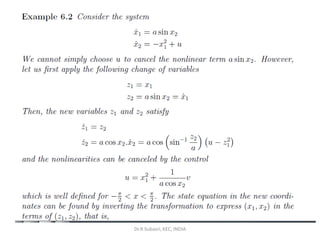
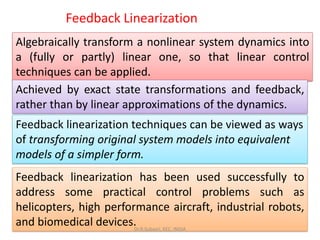
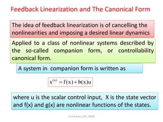
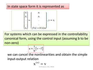
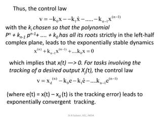
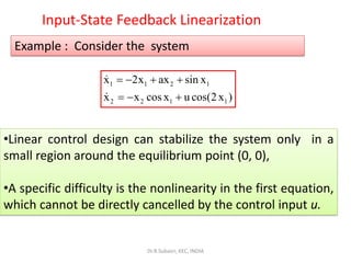
The document discusses feedback linearization, which involves transforming a nonlinear system into an equivalent linear system through state and input transformations. This allows linear control techniques to be applied. Feedback linearization has been successfully used to control helicopters, aircraft, robots, and biomedical devices. It involves finding transformations to cancel the system nonlinearities, resulting in a linear relationship between the transformed input and states. The transformed system can then be stabilized using standard linear control methods like pole placement.
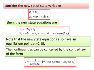


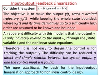
![The dynamic equation of the inverted pendulum is
( ) ( )
1 2
2
1 2 1 1 c 1 c
2 2 2
1 c 1 c
x x
g sinx mlx cos x sin x / (m m) cos x / (m m)
x
l 4 / 3 mcos x / (m m) l 4 / 3 mcos x / (m m)
=
− + +
= +
− + − +
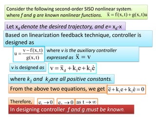
Where x1 and x2 are the oscillation angle and the
oscillation rate respectively. g= 9.8 m/s2 , mc is the
vehicle mass mc = 1 kg, m is the mass of pendulum
bar, m= 0.1 kg, l is one half of pendulum length, l =0.5
m, u is the control input
The desired trajectory is xd (t)= 0.1sin (t). Controller
gains are k1 =k2 =5, The initial state of the inverted
pendulum is [ / 60 0].
Dr.R.Subasri, KEC, INDIA](https://image.slidesharecdn.com/feedbacklinearisation-180810155650/85/Feedback-linearisation-14-320.jpg)
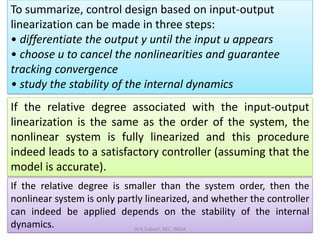
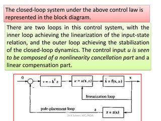
![Feedback Linearisation
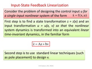
function [sys,x0,str,ts] =
spacemodel(t,x,u,flag)
switch flag,
case 0,
[sys,x0,str,ts]=mdlInitializeSizes;
case 1,
sys=mdlDerivatives(t,x,u);
case 3,
sys=mdlOutputs(t,x,u);
case {1,2,4,9}
sys=[];
otherwise
error(['Unhandled flag = ',
num2str(flag)]);
end
function [sys,x0,str,ts]
=mdlInitializeSizes
sizes = simsizes;
sizes.NumContStates = 0;
sizes.NumDiscStates = 0;
sizes.NumOutputs = 1;
sizes.NumInputs = 5;
sizes.DirFeedthrough = 1;
sizes.NumSampleTimes = 0;
sys = simsizes(sizes);
x0 = [];
str = [];
ts = [];
Dr.R.Subasri, KEC, INDIA](https://image.slidesharecdn.com/feedbacklinearisation-180810155650/85/Feedback-linearisation-15-320.jpg)