Downloaded 551 times
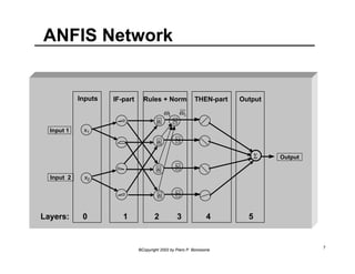
![ANFIS Neurons: Clarification note
• Note that neurons in ANFIS have different
structures:
– Values [ Membership function defined by parameterized
soft trapezoids (Generalized Bell Functions) ]
– Rules [ Differentiable T-norm - usually product ]
– Normalization [ Sum and arithmetic division ]
– Functions [ Linear regressions and multiplication with
, i.e., normalized weights ω, ]
– Output [ Algebraic Sum ]
©Copyright 2002 by Piero P. Bonissone 8
ω](https://image.slidesharecdn.com/anfis-140826050910-phpapp02/85/Anfis-rpi04-8-320.jpg)
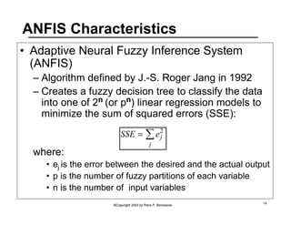

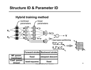
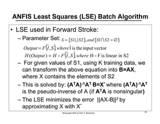
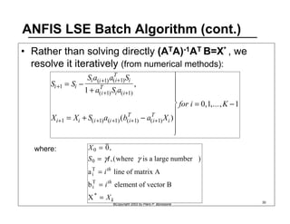
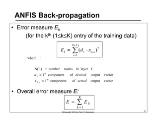
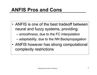

This document provides an overview of Adaptive Neural Fuzzy Inference Systems (ANFIS). It discusses how ANFIS aims to integrate the benefits of fuzzy systems and neural networks by using neural network learning methods to determine the parameters of fuzzy inference systems. The document outlines ANFIS architecture and computational complexity. It also describes how ANFIS uses a hybrid learning algorithm with a least squares estimate to identify linear parameters and backpropagation to adjust nonlinear parameters.