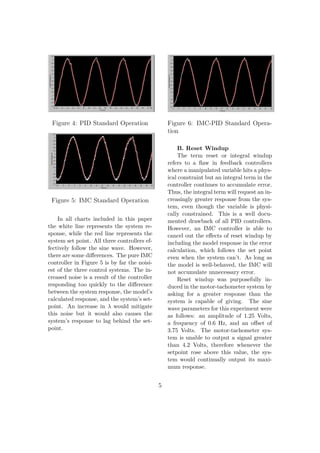
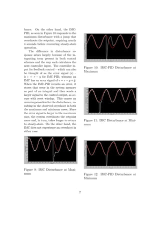
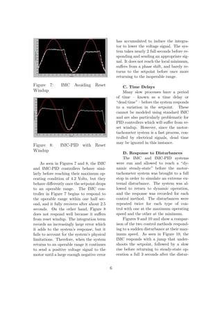
This document summarizes a study comparing three control methods - PID, IMC, and IMC-PID - for controlling a first-order motor-tachometer system. The key findings are: 1) IMC performs better than PID when near system limitations, as PID can exhibit reset windup causing poor control. IMC avoids this issue. 2) Both IMC and IMC-PID effectively control the system under normal operation. However, IMC has less noise than IMC-PID. 3) When a large disturbance occurs, IMC returns to the setpoint faster than IMC-PID, which overshoots due to integral windup.

1. Examining the Benefits of Internal Model Control
in a Motor-Tachometer System
Alexander Harding, Thomas Ignaczak, Logan Williamson, Sammir LeSage
University of Rochester, Rochester NY 14627, March 6, 2017
As technology advances, and manufacturing becomes both cheaper and
more efficient through automation, an understanding of control pro-
cesses has become increasingly valuable. The following project was com-
pleted by the University of Rochester Senior Class of 2017 as part of a
course on Process Dynamics and Control taught by Professor Eldred H.
Chimowitz of the Department of Chemical Engineering. It consists of
controlling a first order motor-tachometer system using three different
control structures. The first control scheme is the PID (Proportional,
Integral, and Derivative) controller, which is commonly used in indus-
try. Another type of control structure is called Internal Model Control
(IMC), which is a model-based scheme that requires insight into the
physical processes. The closer the model is to the actual process, the
better the system behaves. Traditional PID and IMC can be integrated
and shown to be equivalent in many cases, resulting in an IMC-PID
controller. For this project the system’s response for each of the three
methods are compared, then some of the advantages and drawbacks are
investigated. “Pure” IMC performs better than PID-type controllers
when operating at or near system limitations, due to PID controllers
exhibiting reset windup, resulting in poor process control. IMC cal-
culations also allow for the elimination of unnecessary guesswork when
determining characteristic process parameters.
1

2. 1. Internal Model Control Theory
Standard feedback controllers are in-
credibly robust and operate with no in-
formation about the process. IMC at-
tempts to incorporate information known
about the process into a model in order to
establish a precise control method with-
out incorporating PID control parame-
ters.
Figure 1: IMC Block Diagram
By using the Laplace transform, alge-
braic operations can be carried out to es-
tablish equations as a function of the fre-
quency domain (s). Once the equations
have been established an inverse Laplace
transform is used to find the controller
output and system response as functions
of time. See Appendix A for nomencla-
ture.
u(θ) = M(θ) − MMin =
τp
λKp
(r(θ) − y(θ) + ˜y(θ))
+
1
λKp
θ
0
(r(t) − y(t) + ˜y(t))dt
(1)
˜y(θ) =
1
τp
θ
0
{Kpu(t) − ˜y(t)}dt (2)
The controller transfer function of a
PID, c(s), and the controller of an IMC,
q(s), are related through the following
equations:
c(s) =
q(s)
1 − ˜g(s)q(s)
(3)
q(s) =
c(s)
1 + c(s)˜g(s)
(4)
As stated before, IMC and standard
feedback controllers are directly related.
This relationship is illustrated in Figure
2.
Figure 2: Evolution of an IMC Struc-
ture
Figure 3 will show the relation be-
tween the PID, c(s), and the IMC Con-
troller, q(s), are related as shown by
equations 3-4.
Figure 3: Controller Comparison
For the motor-tachometer system,
the first-order process model is:
2

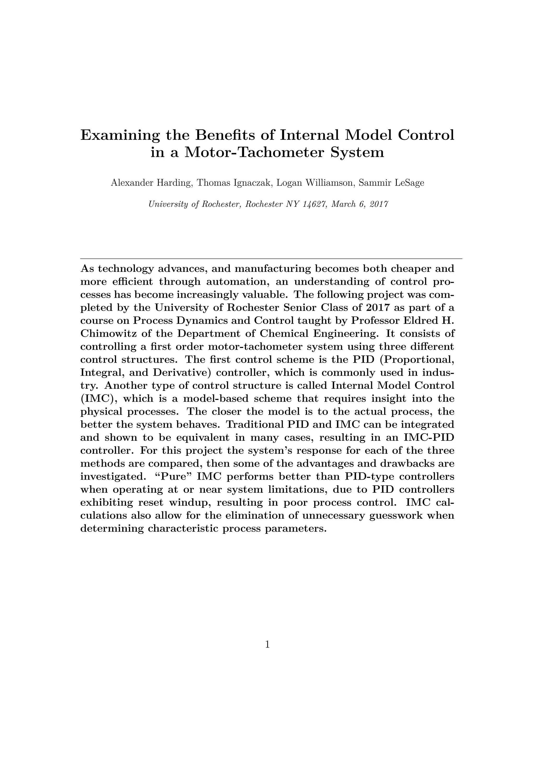
3. ˜g(s) =
Kp
τps + 1
(5)
And the control algorithm for a first-
order process is:
q(s) =
τps + 1
Kp(λs + 1)
(6)
Combining equations 3, 5, and 6 re-
sults in:
c(s) =
τps + 1
λKp
+
1
λKps
(7)
Notice that equation 7 is simply equa-
tion 1 in the frequency domain, and both
are proportional and integral (PI) con-
trollers. The proportional control param-
eter is
τps+1
λKp
and the integration parame-
ter is 1
λKps .
2. The Motor-Tachometer
System
A. Characteristics and
Parameters
It has been shown[2] that a perma-
nent magnet DC motor can be dynam-
ically modeled using the Laplace trans-
form to establish an equation for the
transfer function between an input volt-
age and an output voltage signal. The
motor-tachometer system used in this
project consists of two gears which are
interlocked. One is driven by a signal
from a LabJack between 0 and 5 Volts;
the other is driven by the first, which
is registered by an analog tachometer
as an output voltage signal. The set-
point and the system response are com-
pared in real time using an IMC con-
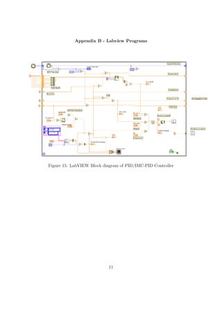
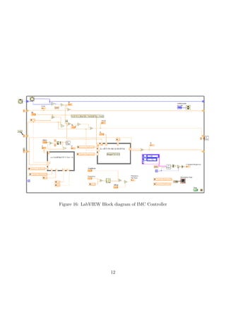
troller and an IMC-PID controller, im-
plemented through LabVIEW programs
found in Appendix B.
Before the programs can be effec-
tively run, there are several characteristic
parameters that must be determined for
the motor-tachometer system: the time
constant, τp, governs the speed of the re-
sponse to changes in the setpoint; the
process gain, Kp, dictates the magnitude
of the response to changes in input volt-
age; and the minimum driving voltage,
MMin, establishes the signal required to
maintain a dynamic state. Additionally,
the motor requires a minimum voltage in
order to overcome static friction and be-
gin dynamic operation. For the given ex-
perimental system, the minimum voltage
is 2.6 Volts.
B. Identifying System
Parameters
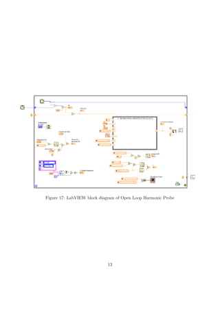
τp, Kp, and MMin are found by first,
probing the system in an open loop with
a known harmonic function, second, de-
veloping a model for how the motor re-
sponds, and, third, carrying out a simple
regression to find the best fitting param-
eters. To ensure dynamic operation, the
motor was set to follow a sinusoidal set-
point established by Equation 8.
M(θ) = Mo + MAsin(ωθ) (8)
Equation 9 establishes a functional
control algorithm for the system to fol-
low the set point.
c(θ) = Kp[(Mo − MMin)[1 − e
−θ
τp ]+
KpMA
τp(ω2 + 1
τ2
p
)
[ωe
−θ
τp +
sin(ωθ + φ)
τpcos(φ)
]
(9)
When the system reaches steady-
state, the exponential decay terms ap-
3

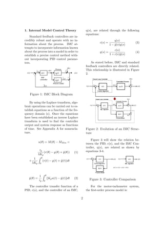
4. proach zero and the response simplifies
to Equation 10.
c(θ) = Kp[(Mo − MMin)+
MA
τ2
p ω2 + 1
sin(ωθ + φ)
cos(φ)
]
(10)
The characteristic parameters τp,
Kp, and MMin were regressed by mini-
mizing the sum of the squared residuals
between the actual system response and
the calculated response using Equation 9.
Table 1 displays the IMC control param-
eters found using this method, and Table
2 displays the IMC parameters found to
work over the widest range of input fre-
quencies and the IMC-PID proportional
and integral control parameters from
them. Also displayed in Table 2 are PID
parameters found empirically.
Table 1: Parameters (top) are fixed
inputs, system characteristics (mid-
dle) are altered to minimize the sum
of the squared residuals (bottom)
between the system response and the
model.
C. Tuning λ
Once the characteristic parameters
of the first-order system are determined,
these values can be used in the IMC al-
gorithm and the program can be exe-
cuted to determine how well the system
responds to a setpoint. The only other
parameter that needs to be tuned is λ,
a tunable time constant for the output
response. As λ is decreased, the system
will respond more quickly to error. How-
ever, for processes where disturbances are
frequent, a small λ may cause the con-
troller to over correct and lead to poor
process control because of this noise am-
plification effect. In these cases, a more
robust model may be needed which will
in effect be able to “ignore” more process
noise. To institute a more robust model,
all that is needed is a larger λ. The opti-
mal value of λ for the motor system was
found to be 0.1, and this value was used
to calculate the IMC-PID parameters in
Table 2.
PID IMC IMC-PID
kp = 1.44 τp = 0.85 kp = 2.17
ki = 2.5 Kp = 3.89 ki = 2.57
kd = 0.30 MMin = 2.43V kd = 0
Table 2. Parameters that yielded best
control
3. Results
A. Comparison of PID, IMC,
and IMC-PID Controllers
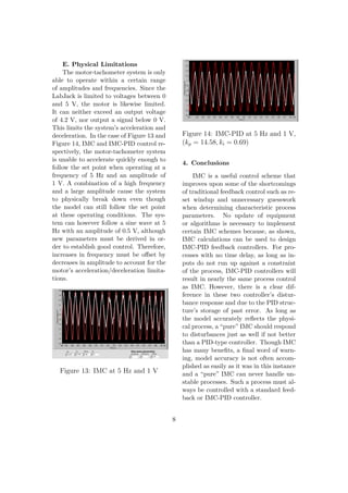
These three control strategies were
compared at the same operating condi-
tions using the parameters in Table 2
to see which gave the most accurate re-
sponse. The conditions were as follows:
after reaching a steady-state the con-
trollers set the motor to follow a sine
wave of frequency 1.2 Hz, amplitude 1.25
Volts, and an offset of 2.75 Volts. At least
two periods at a time were captured in
the following figures.
4

5. Figure 4: PID Standard Operation
Figure 5: IMC Standard Operation
In all charts included in this paper
the white line represents the system re-
sponse, while the red line represents the
system set point. All three controllers ef-
fectively follow the sine wave. However,
there are some differences. The pure IMC
controller in Figure 5 is by far the noisi-
est of the three control systems. The in-
creased noise is a result of the controller
responding too quickly to the difference
between the system response, the model’s
calculated response, and the system’s set-
point. An increase in λ would mitigate
this noise but it would also causes the
system’s response to lag behind the set-
point.
Figure 6: IMC-PID Standard Opera-
tion
B. Reset Windup
The term reset or integral windup
refers to a flaw in feedback controllers
where a manipulated variable hits a phys-
ical constraint but an integral term in the
controller continues to accumulate error.
Thus, the integral term will request an in-
creasingly greater response from the sys-
tem, even though the variable is physi-
cally constrained. This is a well docu-
mented drawback of all PID controllers.
However, an IMC controller is able to
cancel out the effects of reset windup by
including the model response in the error
calculation, which follows the set point
even when the system can’t. As long as
the model is well-behaved, the IMC will
not accumulate unnecessary error.
Reset windup was purposefully in-
duced in the motor-tachometer system by
asking for a greater response than the
system is capable of giving. The sine
wave parameters for this experiment were
as follows: an amplitude of 1.25 Volts,
a frequency of 0.6 Hz, and an offset of
3.75 Volts. The motor-tachometer sys-
tem is unable to output a signal greater
than 4.2 Volts, therefore whenever the
setpoint rose above this value, the sys-
tem would continually output its maxi-
mum response.
5

6. Figure 7: IMC Avoiding Reset
Windup
Figure 8: IMC-PID with Reset
Windup
As seen in Figures 7 and 8, the IMC
and IMC-PID controllers behave simi-
larly before reaching their maximum op-
erating condition of 4.2 Volts, but they
behave differently once the setpoint drops
to an operable range. The IMC con-
troller in Figure 7 begins to respond to
the operable range within one half sec-
ond, and it fully recovers after about 2.5
seconds. On the other hand, Figure 8
does not respond well because it suffers
from reset windup. The integration term
records an increasingly large error which
it adds to the system’s response, but it
fails to account for the system’s physical
limitations. Therefore, when the system
returns to an operable range it continues
to send a positive voltage signal to the
motor until a large enough negative error
has accumulated to induce the integra-
tor to lower the voltage signal. The sys-
tem takes nearly 2 full seconds before re-
sponding and sending an appropriate sig-
nal. It does not reach the local minimum,
suffers from a phase shift, and barely re-
turns to the setpoint before once more
returning to the inoperable range.
C. Time Delays
Many slow processes have a period
of time – known as a time delay or
“dead time” – before the system responds
to a variation in the setpoint. These
cannot be modeled using standard IMC
and are also particularly problematic for
PID controllers which will suffer from re-
set windup. However, since the motor-
tachometer system is a fast process, con-
trolled by electrical signals, dead time
may be ignored in this instance.
D. Response to Disturbances
The IMC and IMC-PID systems
were run and allowed to reach a “dy-
namic steady-state” before the motor-
tachometer system was brought to a full
stop in order to simulate an extreme ex-
ternal disturbance. The system was al-
lowed to return to dynamic operation,
and the response was recorded for each
control method. The disturbances were
repeated twice for each type of con-
trol with one at the maximum operating
speed and the other at the minimum.
Figures 9 and 10 and show a compar-
ison of the two control methods respond-
ing to a sudden disturbance at their max-
imum speed. As seen in Figure 10, the
IMC responds with a jump that under-
shoots the setpoint, followed by a slow
rise before returning to steady-state op-
eration a full 3 seconds after the distur-
6

7. bance. On the other hand, the IMC-
PID, as seen in Figure 10 responds to the
maximum disturbance with a jump that
overshoots the setpoint, requiring nearly
4 seconds before recovering steady-state
operation.
The difference in disturbance re-
sponse arises largely because of the in-
tegrating term present in both control
schemes and the way each calculates the
next controller input. The controller in-
put for feedback control – which can also
be thought of as the error signal ( ) –
is = r − y for IMC-PID, whearas an
IMC has an error signal of = r − y + ˜y.
When the IMC-PID records an error, it
stores that error in the system memory
as part of an integral and then sends a
larger signal to the control output, as oc-
curs with reset windup. This causes an
overcompensation for the disturbance, re-
sulting in the observed overshoot in both
the maximum and minimum cases. Since
the error signal is larger in the maximum
case, the system overshoots the setpoint
more and, in turn, takes longer to return
to steady-state. On the other hand, the
IMC does not experience an overshoot in
either case.
Figure 9: IMC Disturbance at Maxi-
mum
Figure 10: IMC-PID Disturbance at
Maximum
Figure 11: IMC Disturbance at Mini-
mum
Figure 12: IMC-PID Disturbance at
Minimum
7

8. E. Physical Limitations
The motor-tachometer system is only
able to operate within a certain range
of amplitudes and frequencies. Since the
LabJack is limited to voltages between 0
and 5 V, the motor is likewise limited.
It can neither exceed an output voltage
of 4.2 V, nor output a signal below 0 V.
This limits the system’s acceleration and
deceleration. In the case of Figure 13 and
Figure 14, IMC and IMC-PID control re-
spectively, the motor-tachometer system
is unable to accelerate quickly enough to
follow the set point when operating at a
frequency of 5 Hz and an amplitude of
1 V. A combination of a high frequency
and a large amplitude cause the system
to physically break down even though
the model can still follow the set point
at these operating conditions. The sys-
tem can however follow a sine wave at 5
Hz with an amplitude of 0.5 V, although
new parameters must be derived in or-
der to establish good control. Therefore,
increases in frequency must be offset by
decreases in amplitude to account for the
motor’s acceleration/deceleration limita-
tions.
Figure 13: IMC at 5 Hz and 1 V
Figure 14: IMC-PID at 5 Hz and 1 V,
(kp = 14.58, ki = 0.69)
4. Conclusions
IMC is a useful control scheme that
improves upon some of the shortcomings
of traditional feedback control such as re-
set windup and unnecessary guesswork
when determining characteristic process
parameters. No update of equipment
or algorithms is necessary to implement
certain IMC schemes because, as shown,
IMC calculations can be used to design
IMC-PID feedback controllers. For pro-
cesses with no time delay, as long as in-
puts do not run up against a constraint
of the process, IMC-PID controllers will
result in nearly the same process control
as IMC. However, there is a clear dif-
ference in these two controller’s distur-
bance response and due to the PID struc-
ture’s storage of past error. As long as
the model accurately reflects the physi-
cal process, a “pure” IMC should respond
to disturbances just as well if not better
than a PID-type controller. Though IMC
has many benefits, a final word of warn-
ing, model accuracy is not often accom-
plished as easily as it was in this instance
and a “pure” IMC can never handle un-
stable processes. Such a process must al-
ways be controlled with a standard feed-
back or IMC-PID controller.
8

9. References
1) Internal Model Control, Rivera D.
and Flores M.
2) ALTAS, Ismail H. Dynamic Model
of a Permanent Magnet DC Motor. Ka-
radeniz Technical University Faculty of
Engineering Electrical and Electronics En-
gineering Web. 20 Jan. 2017.
9

10. Appendix A - Nomenclature
M(θ): Driving Function
Mo: Offset voltage
MA: wave amplitude
ω: harmonic frequency
θ : Time
c(s): system response
q(s): controller transfer function
u(s) system output
gp(s): process transfer function
˜gp(s): model transfer function
z(s): Setpoint
˜y(s): model output
y(s) system response
φ :phase shift
λ: Filter function constant
s: independent variable of frequency domain
Kp: process gain
kp: proportional constant
ki: integration constant
kd: derivative constant
SSR: Sum of the Squared Residuals AdjSSR: Adjusted Sum of the Squared
Residuals
10

11. Appendix B - Labview Programs
Figure 15: LabVIEW Block diagram of PID/IMC-PID Controller
11

12. Figure 16: LabVIEW Block diagram of IMC Controller
12

13. Figure 17: LabVIEW block diagram of Open Loop Harmonic Probe
13