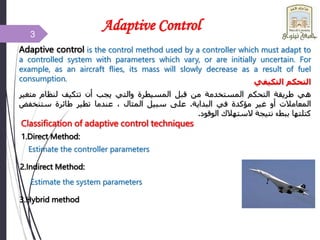
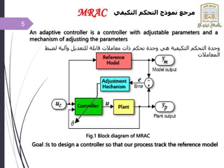
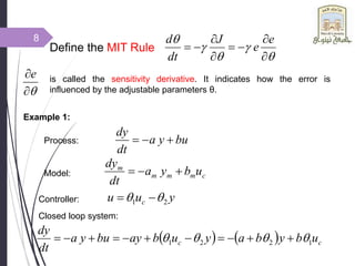
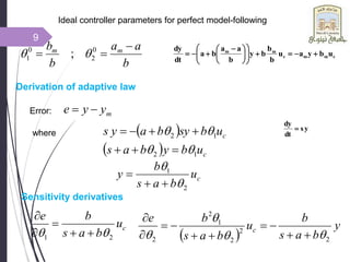
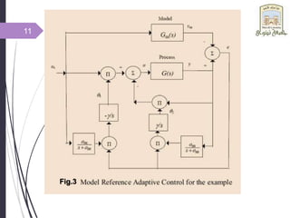
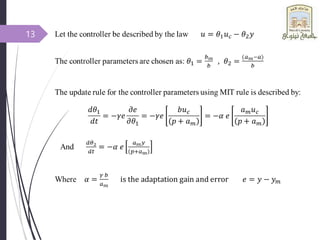
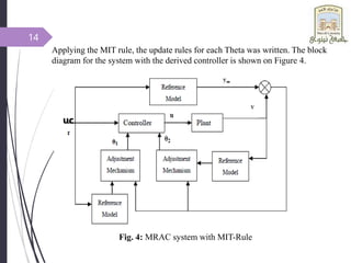
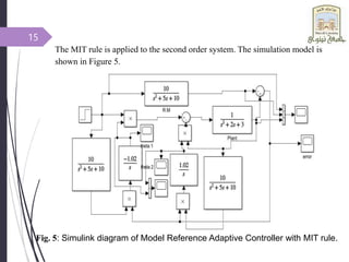
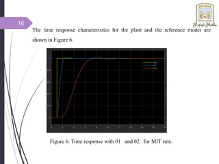
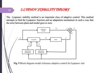
INTRODUCTION TO ADAPTIVE
CONTROL
BY
Mohammed Nawfal Sheet
Hussien Hani Nayef
Muhammad Yasir Adel
Supervised by
Abdullah I. Abdullah
Ali K. Mahmoud
1
Contents
 Adaptive Control
 Why Adaptive Control ?
 MRAC
 MIT Rule
 Design Example
 Lyapunove Rule
 Design example
2
3
Adaptive Control
Adaptive control is the control method used by a controller which must adapt to
a controlled system with parameters which vary, or are initially uncertain. For
example, as an aircraft flies, its mass will slowly decrease as a result of fuel
consumption.
Classification of adaptive control techniques
1.Direct Method:
2.Indirect Method:
3.Hybrid method
Estimate the controller parameters
Estimate the system parameters
‫هي‬
‫طريقة‬
‫التحكم‬
‫المستخدمة‬
‫من‬
‫قبل‬
‫المسيطرة‬
‫والتي‬
‫يجب‬
‫أن‬
‫تتكيف‬
‫لنظام‬
‫متغ‬
‫ير‬
‫المعامالت‬
‫أو‬
‫غير‬
‫مؤكدة‬
‫في‬
‫البداية‬
.
‫على‬
‫سبيل‬
‫المثال‬
،
‫عندما‬
‫تطير‬
‫طائرة‬
‫ستنخفض‬
‫كتلتها‬
‫ببطء‬
‫نتيجة‬
‫الستهالك‬
‫الوقود‬
.
‫التكيفي‬ ‫التحكم‬
4
2.System dynamics experience unpredictable parameter variations
as the control operation goes on
1.Systems to be controlled have parameter uncertainty
Why Adaptive Control ?
Examples
1.Robot manipulation
2.Ship steering
3.Aircraft control
1
.
‫متغيرة‬ ‫معامالت‬ ‫لديها‬ ‫عليها‬ ‫السيطرة‬ ‫يجب‬ ‫التي‬ ‫النظم‬
2
.
‫يمك‬ ‫ال‬ ‫التي‬ ‫المعامالت‬ ‫لتغيرات‬ ‫تتغير‬ ‫النظام‬ ‫استجابة‬
‫التنبؤ‬ ‫ن‬
‫التحكم‬ ‫عملية‬ ‫الستمرار‬ ‫بها‬
‫التكيفي‬ ‫التحكم‬ ‫لماذا‬
5
Fig.1 Block diagram of MRAC
Goal :Is to design a controller so that our process track the reference model
An adaptive controller is a controller with adjustable parameters and a
mechanism of adjusting the parameters
MRAC
‫لض‬ ‫وآلية‬ ‫للتعديل‬ ‫قابلة‬ ‫معامالت‬ ‫ذات‬ ‫تحكم‬ ‫وحدة‬ ‫هي‬ ‫التكيفية‬ ‫التحكم‬ ‫وحدة‬
‫بط‬
‫المعامالت‬
‫التكيفي‬ ‫التحكم‬ ‫نموذج‬ ‫مرجع‬
6
Adjustment of system parameters in a MRAC can be
obtained in two ways.
GRADIENT METHOD (MIT RULE)
LYPNOV STABILITY THEORY
MRAC IS COMPOSED OF
 Plant containing unknown parameters
 Reference model
 Adjustable parameters containing control law
 Ordinary feed back loop
m
y
y
e 

Tracking error:
Introduce the cost function J:   2
2
1
e
J 

Where θ is a vector of controller parameters. Change the parameters in the
direction of the negative gradient of e2.
7
Fig.2 :
1.MIT RULE













e
e
J
dt
d


e is called the sensitivity derivative. It indicates how the error is
influenced by the adjustable parameters θ.
Example 1:
Process: bu
y
a
dt
dy



Model: c
m
m
m
m
u
b
y
a
dt
dy



Controller: y
u
u c 2
1 
 

Closed loop system:
    c
c u
b
y
b
a
y
u
b
ay
bu
y
a
dt
dy
1
2
2
1 


 










Define the MIT Rule
8
Ideal controller parameters for perfect model-following
b
a
a
b
b m
m 

 0
2
0
1 ; 

Derivation of adaptive law
Error: m
y
y
e 

where
c
u
b
a
s
b
y
2
1





 
  c
c
u
b
y
b
a
s
u
b
sy
b
a
y
s
1
2
1
2











Sensitivity derivatives
c
u
b
a
s
b
e
2
1 
 




 
y
b
a
s
b
u
b
a
s
b
e
c
2
2
2
1
2
2 


 









c
m
m
c
m
m
u
b
y
a
u
b
b
b
y
b
a
a
b
a
dt
dy

















 



y
s
dt
dy

9
Approximate    
m
a
s
b
a
s 


 2

where
e
u
a
s
a
s
e
u
a
s
b
t
c
m
m
c
m














 















 



1
1
e
y
a
s
a
s
e
y
a
s
b
t m
m
m






























 



2
2
m
a
b




10
11
Fig.3
12
Example 2:
Let the second order system be described by
13
14
Applying the MIT rule, the update rules for each Theta was written. The block
diagram for the system with the derived controller is shown on Figure 4.
Fig. 4: MRAC system with MIT-Rule
uc
15
The MIT rule is applied to the second order system. The simulation model is
shown in Figure 5.
Fig. 5: Simulink diagram of Model Reference Adaptive Controller with MIT rule.
16
The time response characteristics for the plant and the reference model are
shown in Figure 6.
Figure 6. Time response with θ1 and θ2 for MIT rule.
17
18
Fig. 8. Output error (y-ym) for MIT
19 2.LYPNOV STABILITY THEORY
The Lyapunov stability method is an important class of adaptive control. This method
attempts to find the Lyapunov function and an adaptation mechanism in such a way that
the error between plant and model goes to zero
Fig. 9 Block diagram model reference adaptive control for lyapunov rule
20 Considering, 2nd order Reference Model
And a 2nd order Plant Model:
By subtracting the equation (1) from equation (2), we get,
21 Replacing in equation (5) from equation (3), we get, u
Integrating equation (9) with respect to t, we get,
22
Let the Lyapunov function for the error dynamics,
This function is zero when e is zero and the controller parameters are equal to the correct
values.
For a valid Lyapunov function, time derivative of lyapunov function must be negative.
The derivative is given by e
23
24
Fig.10 Structure Diagram of MRAC for Lyapunov Rule.
r
25
The lyapunove rule is applied to the second order system. The simulation
model is shown in Figure 11.
Fig. 11: Simulink diagram of Model Reference Adaptive Controller
with lyapunove rule.
26 The time response characteristics for the plant and the reference model are shown
in Figure 12.
Figure 12. Time response with θ1 and θ2 for Lyapunov rule.
27
28
Fig. 14 Output error (y-ym) for Lyapunov rule
29
30
Fig. 16 Output error (y-ym) for MIT and Lyapunov rule
31
Rule
Peak Time
(second)
Maximum
Overshoot
(%)
Settling
Time
(second)
θ1 θ2
Lyapunov 1.2 0 0 3.8 0.71 -0.28
MIT Rule 1.2 0 0 4 0.81 -0.18
TABLE I
Time Response Specifications with Lyapunove and MIT for Different
Adaptation Gain.

Model Reference Adaptive Control.ppt

  • 1.
    INTRODUCTION TO ADAPTIVE CONTROL BY MohammedNawfal Sheet Hussien Hani Nayef Muhammad Yasir Adel Supervised by Abdullah I. Abdullah Ali K. Mahmoud 1
  • 2.
    Contents  Adaptive Control Why Adaptive Control ?  MRAC  MIT Rule  Design Example  Lyapunove Rule  Design example 2
  • 3.
    3 Adaptive Control Adaptive controlis the control method used by a controller which must adapt to a controlled system with parameters which vary, or are initially uncertain. For example, as an aircraft flies, its mass will slowly decrease as a result of fuel consumption. Classification of adaptive control techniques 1.Direct Method: 2.Indirect Method: 3.Hybrid method Estimate the controller parameters Estimate the system parameters ‫هي‬ ‫طريقة‬ ‫التحكم‬ ‫المستخدمة‬ ‫من‬ ‫قبل‬ ‫المسيطرة‬ ‫والتي‬ ‫يجب‬ ‫أن‬ ‫تتكيف‬ ‫لنظام‬ ‫متغ‬ ‫ير‬ ‫المعامالت‬ ‫أو‬ ‫غير‬ ‫مؤكدة‬ ‫في‬ ‫البداية‬ . ‫على‬ ‫سبيل‬ ‫المثال‬ ، ‫عندما‬ ‫تطير‬ ‫طائرة‬ ‫ستنخفض‬ ‫كتلتها‬ ‫ببطء‬ ‫نتيجة‬ ‫الستهالك‬ ‫الوقود‬ . ‫التكيفي‬ ‫التحكم‬
  • 4.
    4 2.System dynamics experienceunpredictable parameter variations as the control operation goes on 1.Systems to be controlled have parameter uncertainty Why Adaptive Control ? Examples 1.Robot manipulation 2.Ship steering 3.Aircraft control 1 . ‫متغيرة‬ ‫معامالت‬ ‫لديها‬ ‫عليها‬ ‫السيطرة‬ ‫يجب‬ ‫التي‬ ‫النظم‬ 2 . ‫يمك‬ ‫ال‬ ‫التي‬ ‫المعامالت‬ ‫لتغيرات‬ ‫تتغير‬ ‫النظام‬ ‫استجابة‬ ‫التنبؤ‬ ‫ن‬ ‫التحكم‬ ‫عملية‬ ‫الستمرار‬ ‫بها‬ ‫التكيفي‬ ‫التحكم‬ ‫لماذا‬
  • 5.
    5 Fig.1 Block diagramof MRAC Goal :Is to design a controller so that our process track the reference model An adaptive controller is a controller with adjustable parameters and a mechanism of adjusting the parameters MRAC ‫لض‬ ‫وآلية‬ ‫للتعديل‬ ‫قابلة‬ ‫معامالت‬ ‫ذات‬ ‫تحكم‬ ‫وحدة‬ ‫هي‬ ‫التكيفية‬ ‫التحكم‬ ‫وحدة‬ ‫بط‬ ‫المعامالت‬ ‫التكيفي‬ ‫التحكم‬ ‫نموذج‬ ‫مرجع‬
  • 6.
    6 Adjustment of systemparameters in a MRAC can be obtained in two ways. GRADIENT METHOD (MIT RULE) LYPNOV STABILITY THEORY MRAC IS COMPOSED OF  Plant containing unknown parameters  Reference model  Adjustable parameters containing control law  Ordinary feed back loop
  • 7.
    m y y e   Tracking error: Introducethe cost function J:   2 2 1 e J   Where θ is a vector of controller parameters. Change the parameters in the direction of the negative gradient of e2. 7 Fig.2 : 1.MIT RULE
  • 8.
                 e e J dt d   e is calledthe sensitivity derivative. It indicates how the error is influenced by the adjustable parameters θ. Example 1: Process: bu y a dt dy    Model: c m m m m u b y a dt dy    Controller: y u u c 2 1     Closed loop system:     c c u b y b a y u b ay bu y a dt dy 1 2 2 1                Define the MIT Rule 8
  • 9.
    Ideal controller parametersfor perfect model-following b a a b b m m    0 2 0 1 ;   Derivation of adaptive law Error: m y y e   where c u b a s b y 2 1          c c u b y b a s u b sy b a y s 1 2 1 2            Sensitivity derivatives c u b a s b e 2 1          y b a s b u b a s b e c 2 2 2 1 2 2               c m m c m m u b y a u b b b y b a a b a dt dy                       y s dt dy  9
  • 10.
    Approximate    m a s b a s     2  where e u a s a s e u a s b t c m m c m                                     1 1 e y a s a s e y a s b t m m m                                    2 2 m a b     10
  • 11.
  • 12.
    12 Example 2: Let thesecond order system be described by
  • 13.
  • 14.
    14 Applying the MITrule, the update rules for each Theta was written. The block diagram for the system with the derived controller is shown on Figure 4. Fig. 4: MRAC system with MIT-Rule uc
  • 15.
    15 The MIT ruleis applied to the second order system. The simulation model is shown in Figure 5. Fig. 5: Simulink diagram of Model Reference Adaptive Controller with MIT rule.
  • 16.
    16 The time responsecharacteristics for the plant and the reference model are shown in Figure 6. Figure 6. Time response with θ1 and θ2 for MIT rule.
  • 17.
  • 18.
    18 Fig. 8. Outputerror (y-ym) for MIT
  • 19.
    19 2.LYPNOV STABILITYTHEORY The Lyapunov stability method is an important class of adaptive control. This method attempts to find the Lyapunov function and an adaptation mechanism in such a way that the error between plant and model goes to zero Fig. 9 Block diagram model reference adaptive control for lyapunov rule
  • 20.
    20 Considering, 2ndorder Reference Model And a 2nd order Plant Model: By subtracting the equation (1) from equation (2), we get,
  • 21.
    21 Replacing inequation (5) from equation (3), we get, u Integrating equation (9) with respect to t, we get,
  • 22.
    22 Let the Lyapunovfunction for the error dynamics, This function is zero when e is zero and the controller parameters are equal to the correct values. For a valid Lyapunov function, time derivative of lyapunov function must be negative. The derivative is given by e
  • 23.
  • 24.
    24 Fig.10 Structure Diagramof MRAC for Lyapunov Rule. r
  • 25.
    25 The lyapunove ruleis applied to the second order system. The simulation model is shown in Figure 11. Fig. 11: Simulink diagram of Model Reference Adaptive Controller with lyapunove rule.
  • 26.
    26 The timeresponse characteristics for the plant and the reference model are shown in Figure 12. Figure 12. Time response with θ1 and θ2 for Lyapunov rule.
  • 27.
  • 28.
    28 Fig. 14 Outputerror (y-ym) for Lyapunov rule
  • 29.
  • 30.
    30 Fig. 16 Outputerror (y-ym) for MIT and Lyapunov rule
  • 31.
    31 Rule Peak Time (second) Maximum Overshoot (%) Settling Time (second) θ1 θ2 Lyapunov1.2 0 0 3.8 0.71 -0.28 MIT Rule 1.2 0 0 4 0.81 -0.18 TABLE I Time Response Specifications with Lyapunove and MIT for Different Adaptation Gain.