This document provides an overview of exponential random graph models (ERGMs) for statistically modeling social networks. It discusses the goals of using ERGMs, which are to understand structural features of networks, test hypotheses about network formation processes, and link macro network structures to micro behaviors. Example model terms that can be used in ERGMs are described, ranging from simple models with just edges to more complex models incorporating triangles, degree distributions, and homophily. The document outlines the challenges of estimating ERGM parameters using maximum likelihood due to the normalizing constant, and notes that simulation-based approximations are typically used instead.

1. Exponential Random Graph Models
(ERGM)
Jeffrey A. Smith
University of Nebraska-Lincoln
Department of Sociology
Social Networks & Health Workshop
May 19, 2016

2. The Macro Structure of the Session(s)
n Introduction to ERGMs (1 hour and 15 minutes)
n Introduction to the model
n Estimation
n Hands on approach to modeling networks using
ERGM (1 hour and 30 minutes)
n A quick review of R (data management, network objects…)
n Describing and visualizing the network
n Fitting the network using statnet
• Model terms and constraints
• Interpretation
n Checking the diagnostics of the model
n Checking model fit

3. Goals
n Have a basic sense of ERGMs
n What they are and what you can do with them
n Be able to fit an ERGM to your data
n Be able to tell if the algorithm “worked”
n Be able to tell if the model was a good one
n Run the model, know what it means, know if
there are any problems

4. Introduction to ERGM
n Introduction
n Why statistically model a network?
n Introduce the exponential family
n Some example models: simple to complex
n Estimation

5. Some Preliminaries
n Formally: a network is a set of n nodes
and the social relationships between each
pair of nodes.
n For each pair of actors, or nodes, i,j in the set
N (N=1,2…n), let Yij= 1 if there exists a tie
from i to j and Yij=0 if no tie exists
n Assume here that we are working with
complete network data
n But can run ERGMs using sample data
(Morris and Krivistky et al. 2011; Smith 2012)

6. Slide Credit: James Moody
Why Statistically Model a Network?

9. Figure 1. The largest connected component of
One mesoscopic s
consists of a grou
densely connected
nected to other de
We illustrate this
known benchmark
literature [131].
The existence o
itively clear, and th
have been studied
ogy [25, 44, 79] and
For example, Stua
to investigate poli
and George Homa
of rearranging th
matrices to reveal
1950 [60]. Robert W
formed (using org
have been the firs
nity structure in 1
espoused surprisin
ty structure and co
1960s [117]. Socia
arising in the flo
cial organizations
Coauthorship between
scholars in physics literature
Slide Credit: Porter et al. 2009

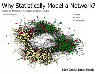
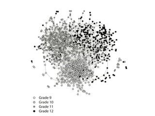
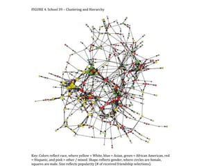
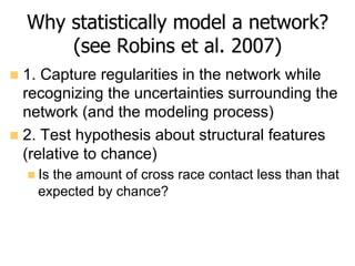
10. Why statistically model a network?
(see Robins et al. 2007)
n 1. Capture regularities in the network while
recognizing the uncertainties surrounding the
network (and the modeling process)
n 2. Test hypothesis about structural features
(relative to chance)
n Is the amount of cross race contact less than that
expected by chance?

11. Why statistically model a network?
(see Robins et al. 2007)
n 3. Test competing hypothesis about
process of network generation
n transitivity versus homophily in generating
group structure
n 4. Macro-micro link
n Can we specify the local processes that
generate the features of the whole network?

12. Example Health Related Questions
We Could Answer
n Are popular (high status) adolescents more
likely to drink, smoke, etc?
n Are people who smoke/drink, etc. more likely
to be friends with others who smoke/ drink?
n How much of this tendency is due to transitive
closure and reciprocity?

13. Example Health Related Questions
We Could Answer
n What processes determine whom one goes to
for health advice?
n How prone is the network to epidemics?
n spread of HIV, HCV
n How effective are different interventions likely
to be?

14. A word of warning
n 1. Fancy network models are not a
substitute for asking good, interesting
questions
n 2. The following discussion has many
formulas and some technical details. The
details are not critical for actually running
the models. The key is to have some
sense of what the models do and the
terms you can use in them. We will get to
the hands on portion in short order.

15. The Exponential Family
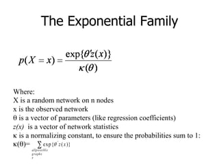
Where:
X is a random network on n nodes
x is the observed network
θ is a vector of parameters (like regression coefficients)
z(x) is a vector of network statistics
κ is a normalizing constant, to ensure the probabilities sum to 1:
κ (θ)= ∑
x
graphs
eallpossibl
xz )}(exp{ '
θ

16. p(X=x)
n The dependent variable is all ij pairs in the
network
n Trying to predict the presence or absence
of ties between pairs of nodes in x
n In other words:
n Each possible network tie is a random
variable
n Predicting ties between i and j probabilistically

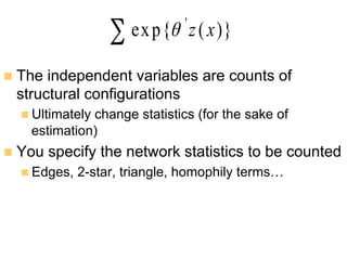
17. n The independent variables are counts of
structural configurations
n Ultimately change statistics (for the sake of
estimation)
n You specify the network statistics to be counted
n Edges, 2-star, triangle, homophily terms…
∑ )}(exp{ '
xzθ

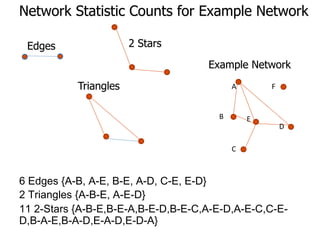
18. 6 Edges {A-B, A-E, B-E, A-D, C-E, E-D}
2 Triangles {A-B-E, A-E-D}
11 2-Stars {A-B-E,B-E-A,B-E-D,B-E-C,A-E-D,A-E-C,C-E-
D,B-A-E,B-A-D,E-A-D,E-D-A}
A
B
C
E
F
D
Edges 2 Stars
Triangles
Example Network
Network Statistic Counts for Example Network

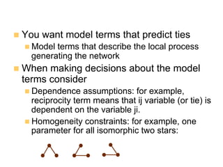
19. n You want model terms that predict ties
n Model terms that describe the local process
generating the network
n When making decisions about the model
terms consider
n Dependence assumptions: for example,
reciprocity term means that ij variable (or tie) is
dependent on the variable ji.
n Homogeneity constraints: for example, one
parameter for all isomorphic two stars:

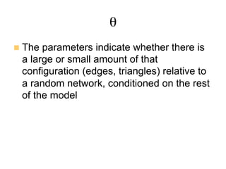
20. θ
n The parameters indicate whether there is
a large or small amount of that
configuration (edges, triangles) relative to
a random network, conditioned on the rest
of the model

21. K(θ)
n Normalizing constant
n More on this when we get to estimation

22. Some example Models: Simple to Complex
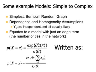
n Simplest: Bernoulli Random Graph
n Dependence and Homogeneity Assumptions
n Yij are independent and all equally likely
n Equates to a model with just an edge term
(the number of ties in the network)
)(
}{exp
)(
,
θκ
θ ∑
==
ji
ijx
xXp
Written as:

23. Dyadic Independent Models
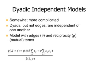
n Somewhat more complicated
n Dyads, but not edges, are independent of
one another
n Model with edges (θ) and reciprocity (ρ)
(mutual) terms
),(
)exp()(
,,
ρθ
ρθ
k
xxxxXp
ji
jiij
ji
ij ∑∑ +==

24. Dyadic Independent Models: p1
(Holland and Leinhardt-1981)
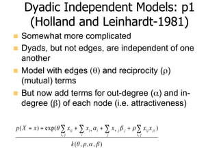
n Somewhat more complicated
n Dyads, but not edges, are independent of one
another
n Model with edges (θ) and reciprocity (ρ)
(mutual) terms
n But now add terms for out-degree (α) and in-
degree (β) of each node (i.e. attractiveness)
),,,(
)exp()(
,,
βαρθ
ρβαθ
k
xxxxxxXp
ji
jiijj
j
ji
i
i
ji
ij ∑∑∑∑ +++== ++

25. Dyadic Independent Models
n Can add terms for homophily
n Ties more likely if i and j share some
characteristic
n Drop homogeneity assumption=differential
homophily (ties are more likely if i and j share
a characteristic, but more true for some
groups than others)
n Nodal characteristics instead of dummies
for each person (for example, do girls
have fewer ties than boys?)

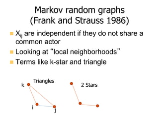
26. Markov random graphs
(Frank and Strauss 1986)
n Xij are independent if they do not share a
common actor
n Looking at “local neighborhoods”
n Terms like k-star and triangle
2 Stars
Triangles
i j
k

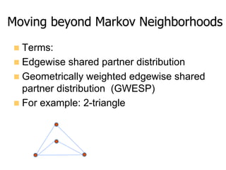
27. n Terms:
n Edgewise shared partner distribution
n Geometrically weighted edgewise shared
partner distribution (GWESP)
n For example: 2-triangle
Moving beyond Markov Neighborhoods

28. n Higher order terms like GWESP often lead
to better model fit (more on this later)
n But are they easily interpretable?
Moving beyond Markov Neighborhoods

29. List of Typical Terms
n Edges
n Mutuality
n Attractiveness/expansiveness
n Homophily (match, differential, mixing)
n Nodefactor
n Edge-covariates
n Degree distribution
n Triangles
n 2-stars
n Cycles
n GWESP

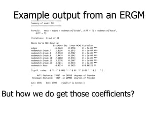
30. Example output from an ERGM
But how we do get those coefficients?
Null Deviance: 28987 on 20910 degrees of freedom
Residual Deviance: 1919 on 20902 degrees of freedom
AIC: 1935 BIC: 1999 (Smaller is better.)
>
> summary(fauxmodel.01)
==========================
Summary of model fit
==========================
Formula: mesa ~ edges + nodematch("Grade", diff = T) + nodematch("Race",
diff = F)
Iterations: 8 out of 20
Monte Carlo MLE Results:
Estimate Std. Error MCMC % p-value
edges -6.2228 0.1738 0 < 1e-04 ***
nodematch.Grade.7 2.8256 0.1975 0 < 1e-04 ***
nodematch.Grade.8 2.9148 0.2382 0 < 1e-04 ***
nodematch.Grade.9 2.4474 0.2642 0 < 1e-04 ***
nodematch.Grade.10 2.6080 0.3743 0 < 1e-04 ***
nodematch.Grade.11 3.3376 0.2967 0 < 1e-04 ***
nodematch.Grade.12 3.7041 0.4573 0 < 1e-04 ***
nodematch.Race 0.4214 0.1435 0 0.00333 **
---
Signif. codes: 0 ‘***’ 0.001 ‘**’ 0.01 ‘*’ 0.05 ‘.’ 0.1 ‘ ’ 1
Null Deviance: 28987 on 20910 degrees of freedom
Residual Deviance: 1919 on 20902 degrees of freedom
AIC: 1935 BIC: 1999 (Smaller is better.)
>

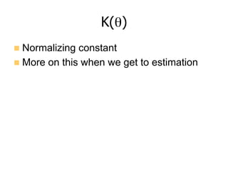
31. Estimation
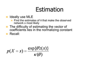
n Ideally use MLE
n Find the estimates of θ that make the observed
network x most likely
n The difficulty of estimating the vector of
coefficients lies in the normalizing constant
n Recall:

32. n To estimate coefficient values by MLE, we
need to know something about the distribution of graph
statistics across “all possible networks”
n But this is difficult as there are a very large number of
possible networks-can’t enumerate them all

33. MLE Estimation
n Likelihood formula:
n Want to estimate unknown parameters ,θ, given the
observed network
n Can’t get ML estimates directly (because the
normalizing constant can’t be enumerated) so
approximate by simulation
Journal of Statistical Software
aximize `(✓) directly, we will consider instead the log-ratio of likelihood v
`(✓) `(✓0) = (✓ ✓0)>
g(yobs) log

(✓, Y)
(✓0, Y)
,
arbitrarily chosen parameter vector. [Note: Previously in this article, we
the term “coe cient” in situations in which either “coe cient” or “param
ally be correct. To be precise, a coe cient in this context is a specific
namely, one that is multiplied by a statistic as in this case or in the
enerally. In this section, we may use the terms “parameter” and “coe
y.]
ation of ratios of normalizing constants such as the one in expression (
well-studied problem (Meng and Wong 1996; Gelman and Meng 1998).
xploit in the ergm function is due to Geyer and Thompson (1992) and m
llows: Starting from Equations 1 and 2, a bit of algebra reveals that
(✓, Y) n
>
o

34. Markov Chain Monte Carlo MLE
(MCMCMLE)
n A somewhat complicated process so we
won’t go into detail, just the basics so we
can tell if something hasn’t gone well

35. Markov Chain Monte Carlo MLE
(MCMCMLE)
n Basic Idea:
n When model includes dyad dependent terms,
use MCMC estimation
n Simulate a set of networks to use as sample
n Necessary to approximate unknown part of
likelihood (k(θ))
n Gibbs Sampling (or Metropolis)

36. The Problem of Degeneracy
n Some parameter values will generate a sample
of networks (the MCMC sample) with probability
mass on 1 or only a few networks
n Often complete or empty network
n Can’t get MLE estimates under such conditions
n Problems with triangle and other markov
neighborhood terms
n GWESP and similar terms less likely to have
such problems (Snidjer et al. 2006)

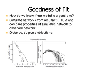
37. Goodness of Fit
n How do we know if our model is a good one?
n Simulate networks from resultant ERGM and
compare properties of simulated network to
observed network
n Distance, degree distributions