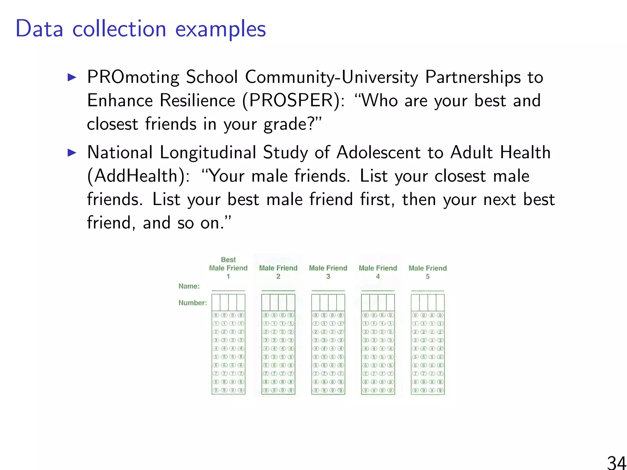
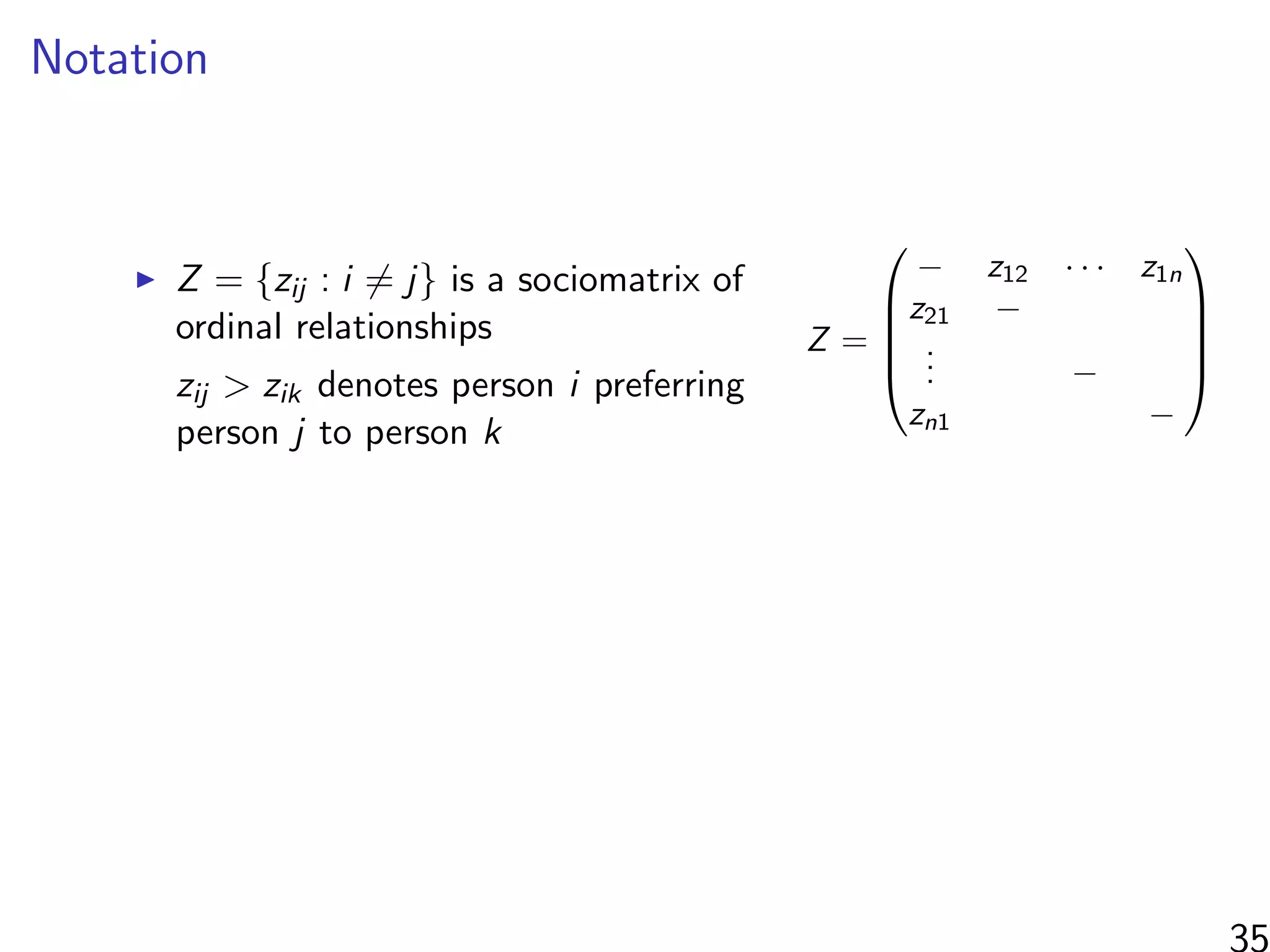
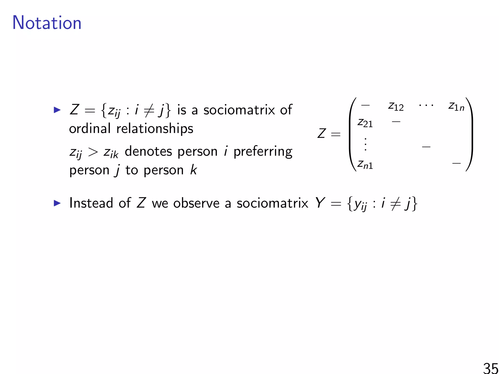
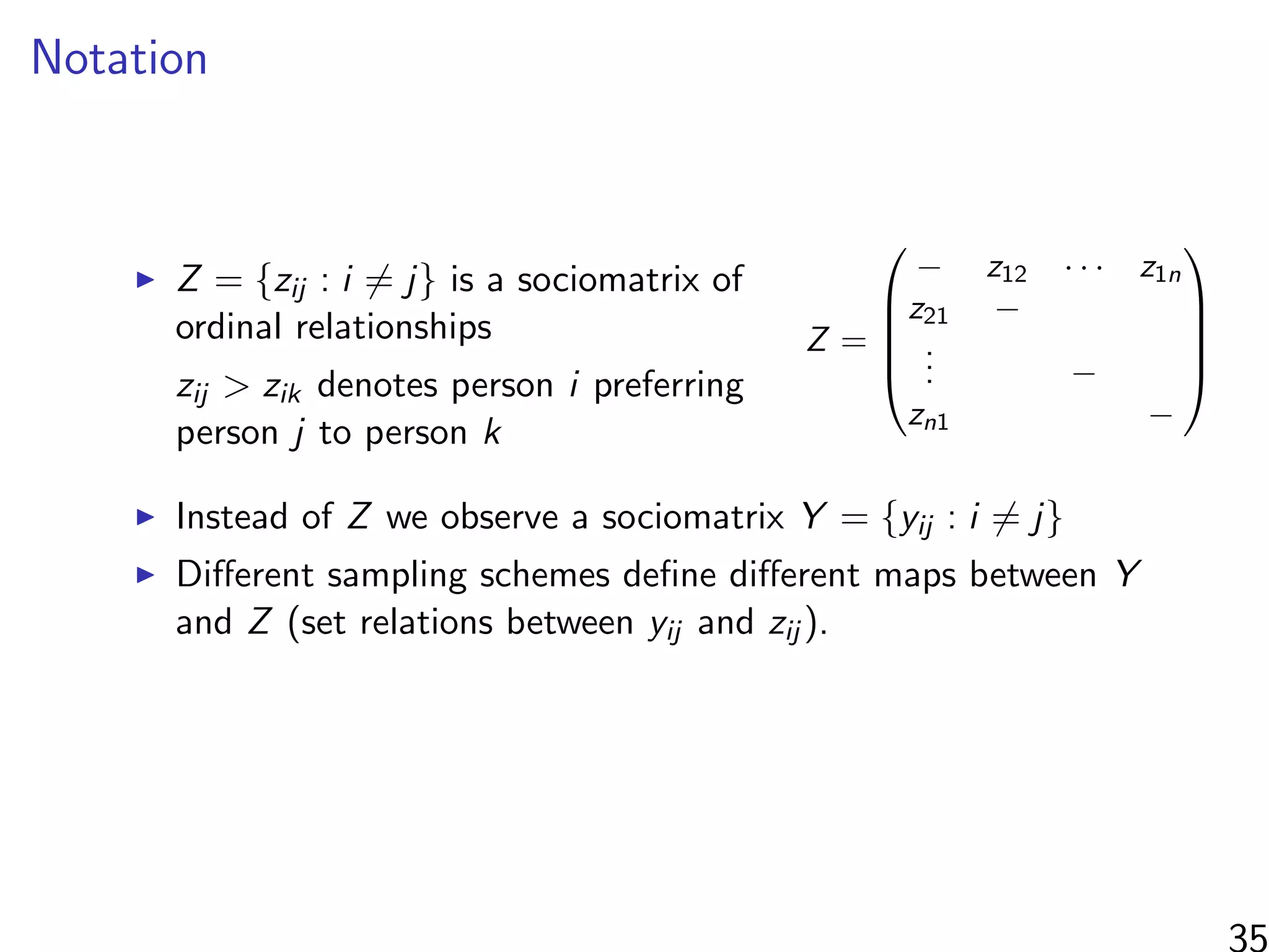
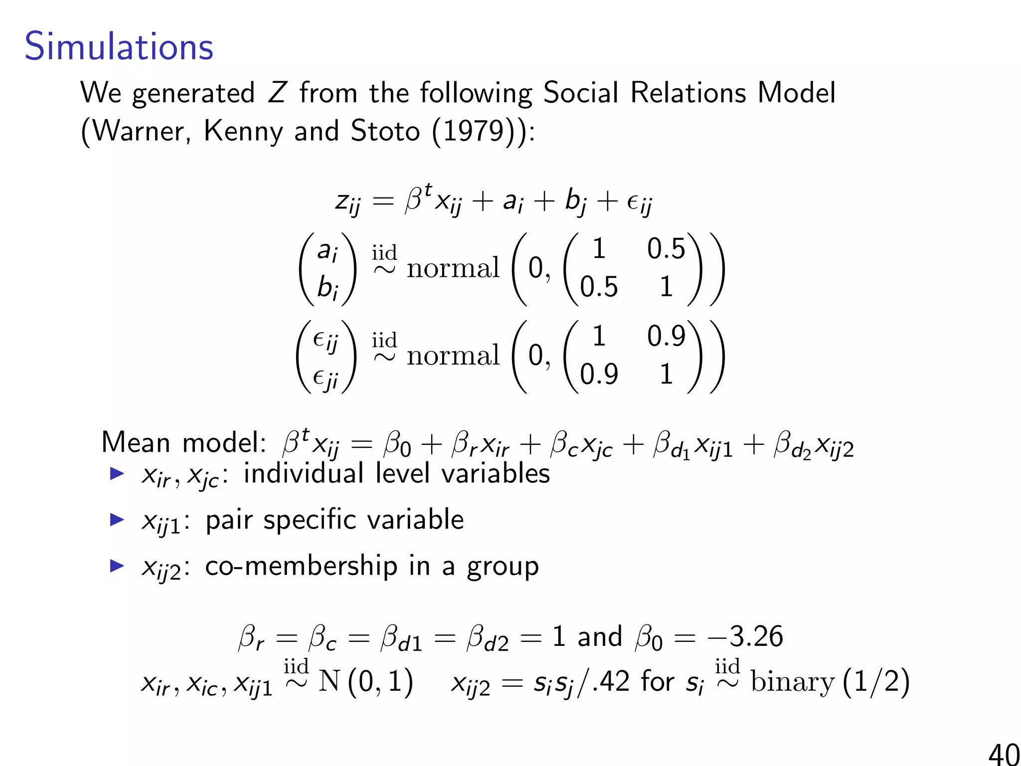
This document discusses modeling networks using regression analysis with additive and multiplicative effects. It introduces network modeling and describes some common network regression models, including the social relations model (SRM) which captures sender and receiver effects. The document discusses incorporating covariates into these models and using multiplicative effects to better capture triadic behavior and homophily in networks. It also briefly mentions generalizing these models to ordinal outcomes.
![How do they solve it?
Interested in estimating
1
N
N
i=1
[Yi (all treated) − Yi (all controls)]
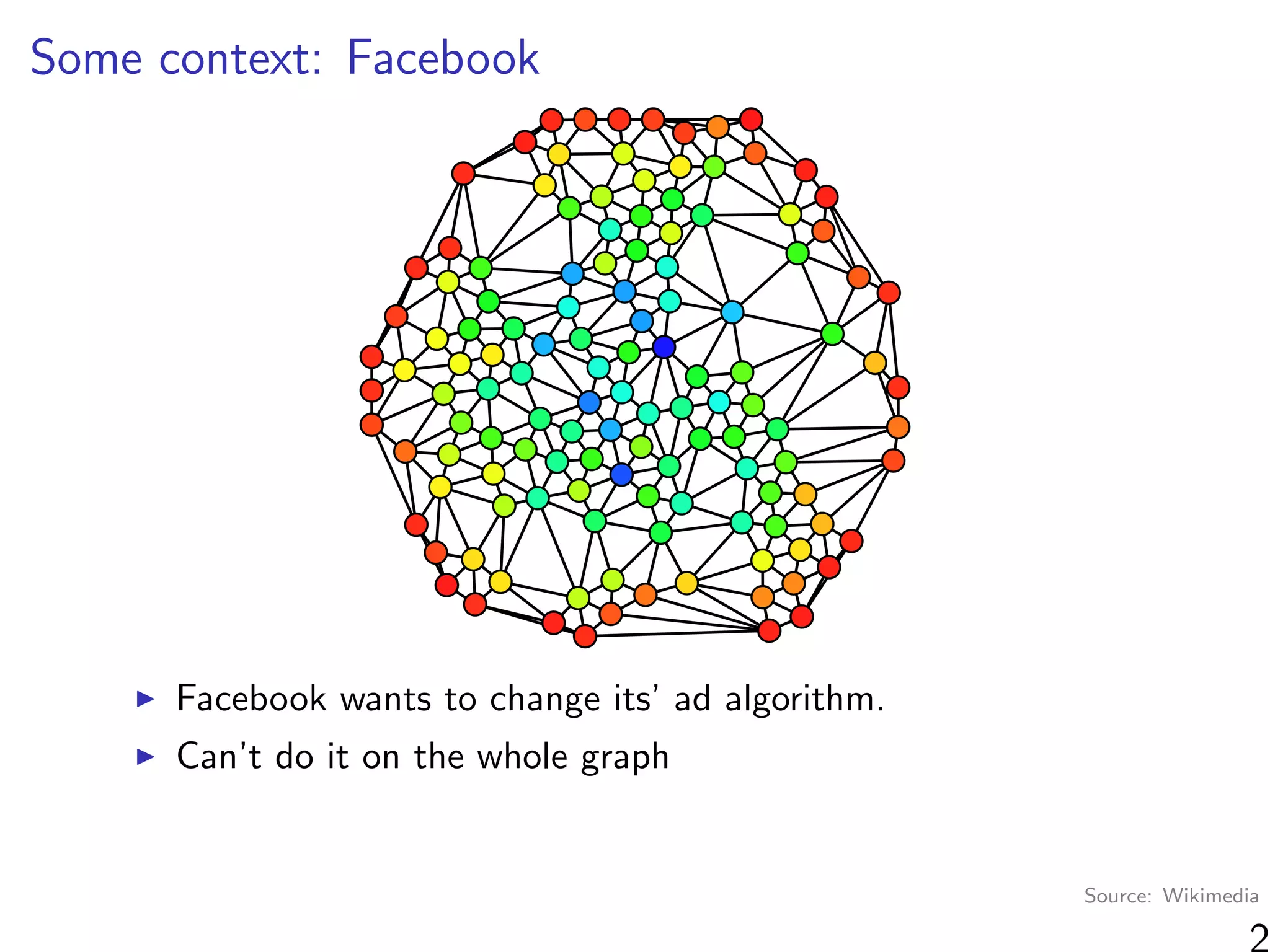
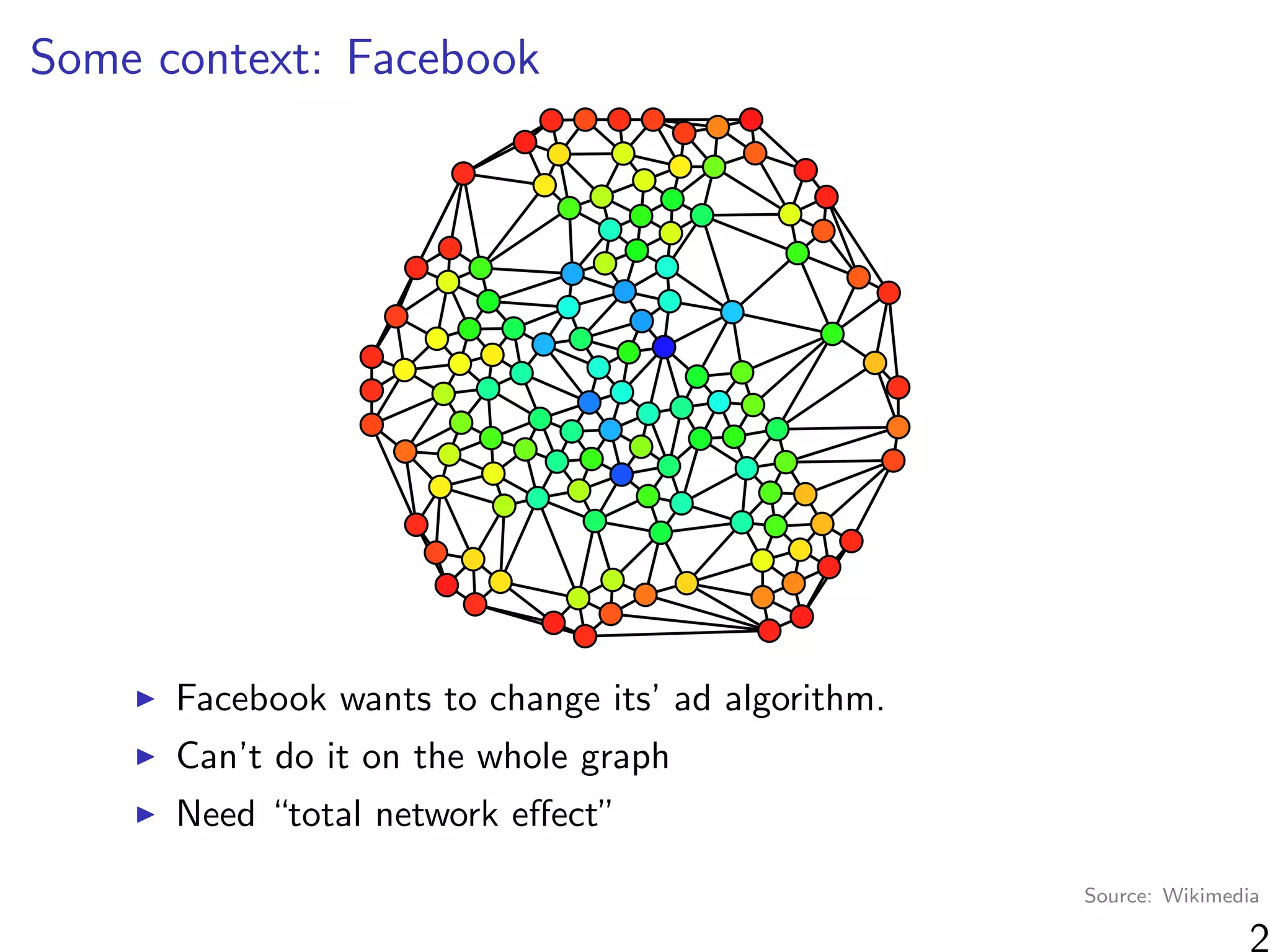
“At a high level, graph cluster randomization is a technique in
which the graph is partitioned into a set of clusters, and then
randomization between treatment and control is performed at
the cluster level.”
Where can we find clusters?
Observable information (e.g. same school)
Unobservable information (“social space”)
3](https://image.slidesharecdn.com/thursdaymorninglecture-latentspacemodels-170629153330/75/08-Inference-for-Networks-DYAD-Model-Overview-2017-14-2048.jpg)


![Simulations - information in the ranks
Same setup as before, but average uncensored outdegree is m
10 20 30 40 50
0.20.40.60.81.01.21.4
m
relativeconcentrationaroundtruevalue
! ! !
! !r
!
!
! ! !c
!
!
!
! !d1
! !
!
! !d2
2: Posterior concentration around true parameter values. The average of E[(β −
(S)]/E[(β − β∗)2|C(S)] across eight simulated datasets for each m ∈ {5, 15, 30, 50}.
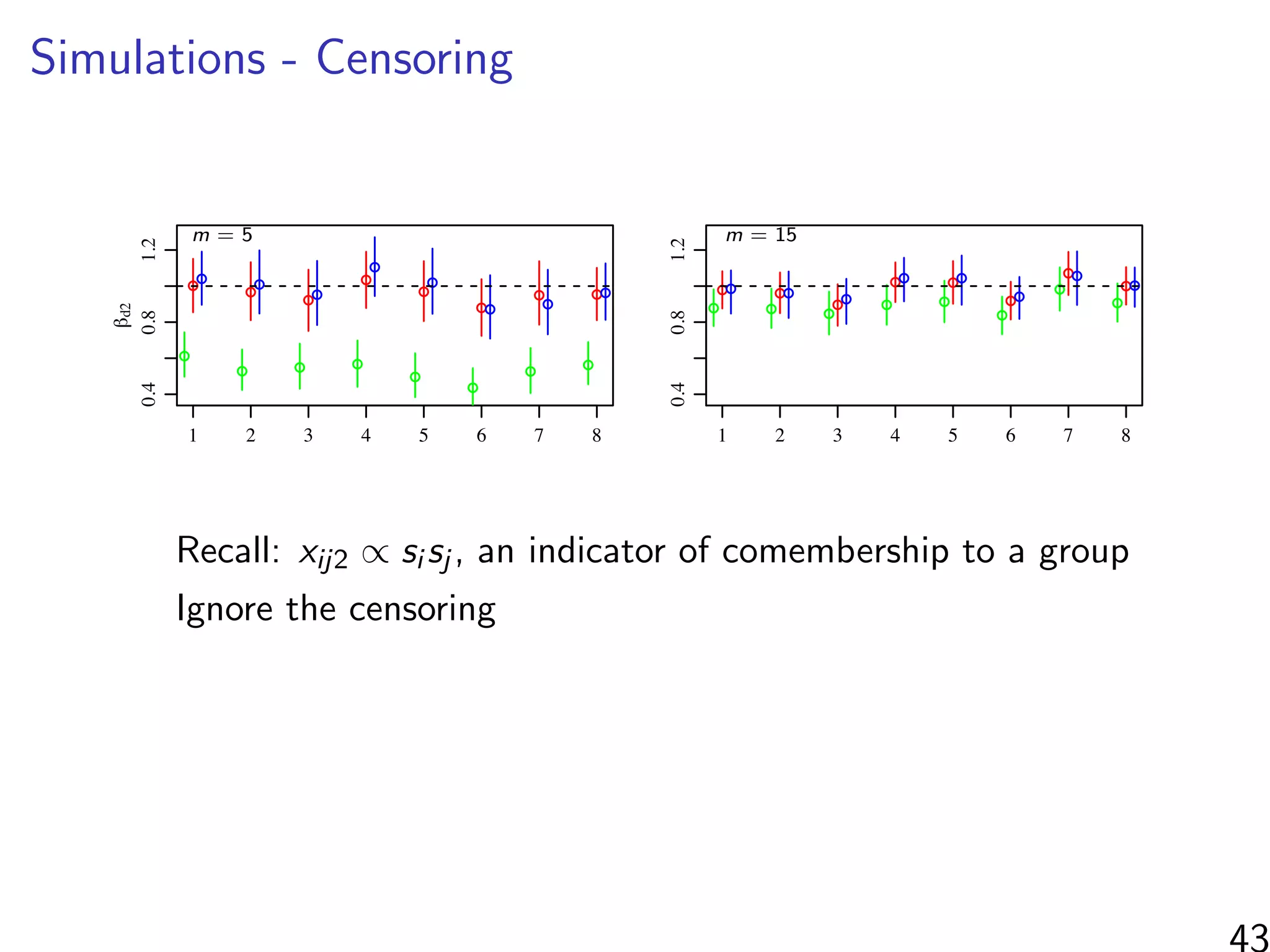
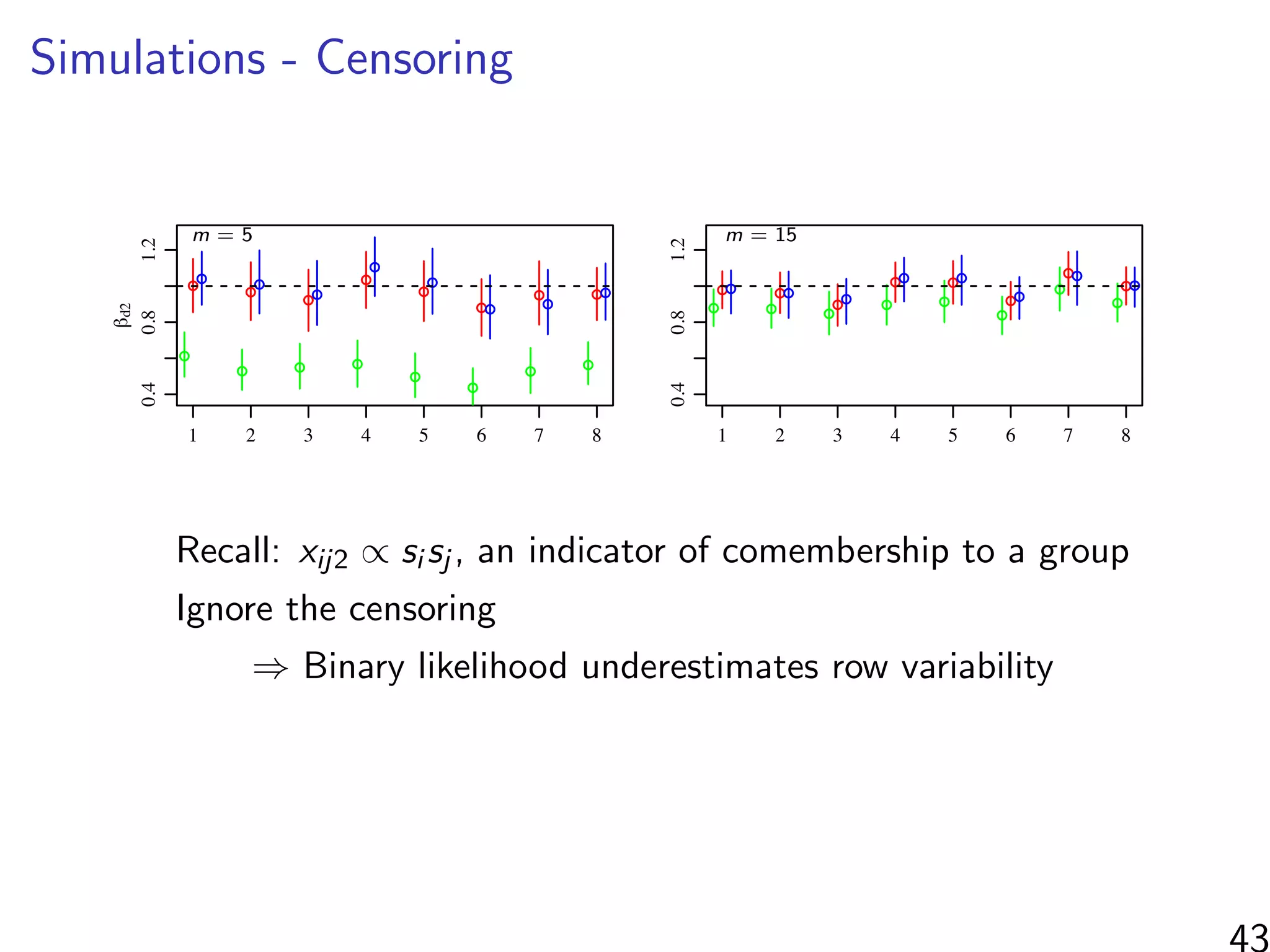
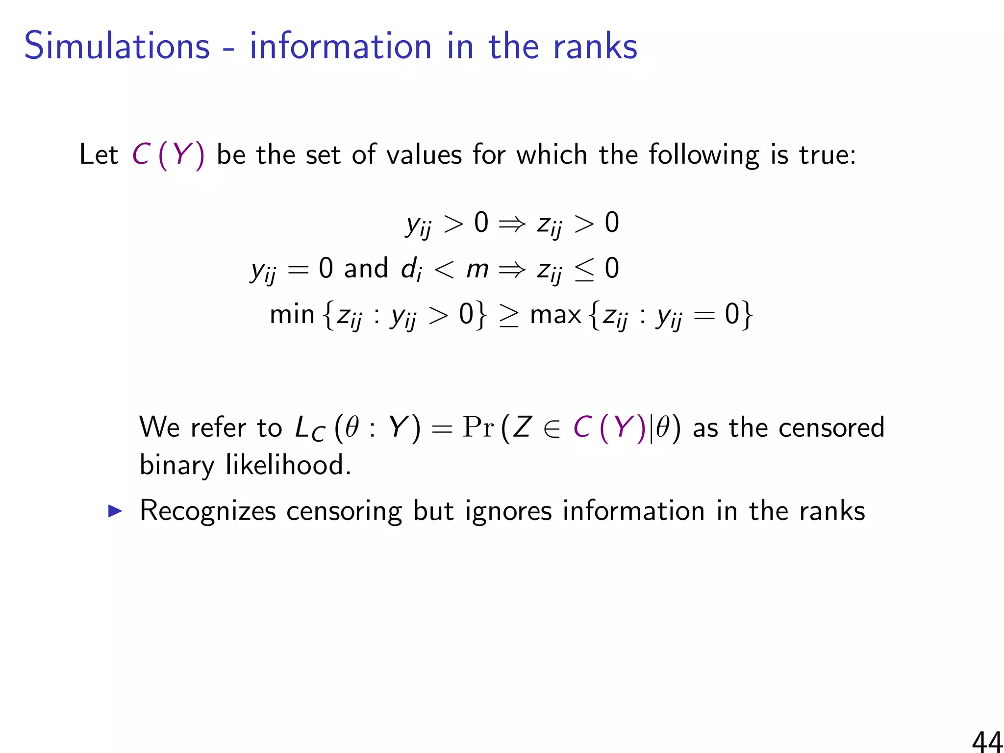
censored binomial likelihood. As the censored binomial likelihood recognizes the censoring in
data, we expect it to provide parameter estimates that do not have the biases of the binomial
ood estimators. On the other hand, LC ignores the information in the ranks of the scored
duals, and so we might expect it to provide less precise estimates than the FRN likelihood.
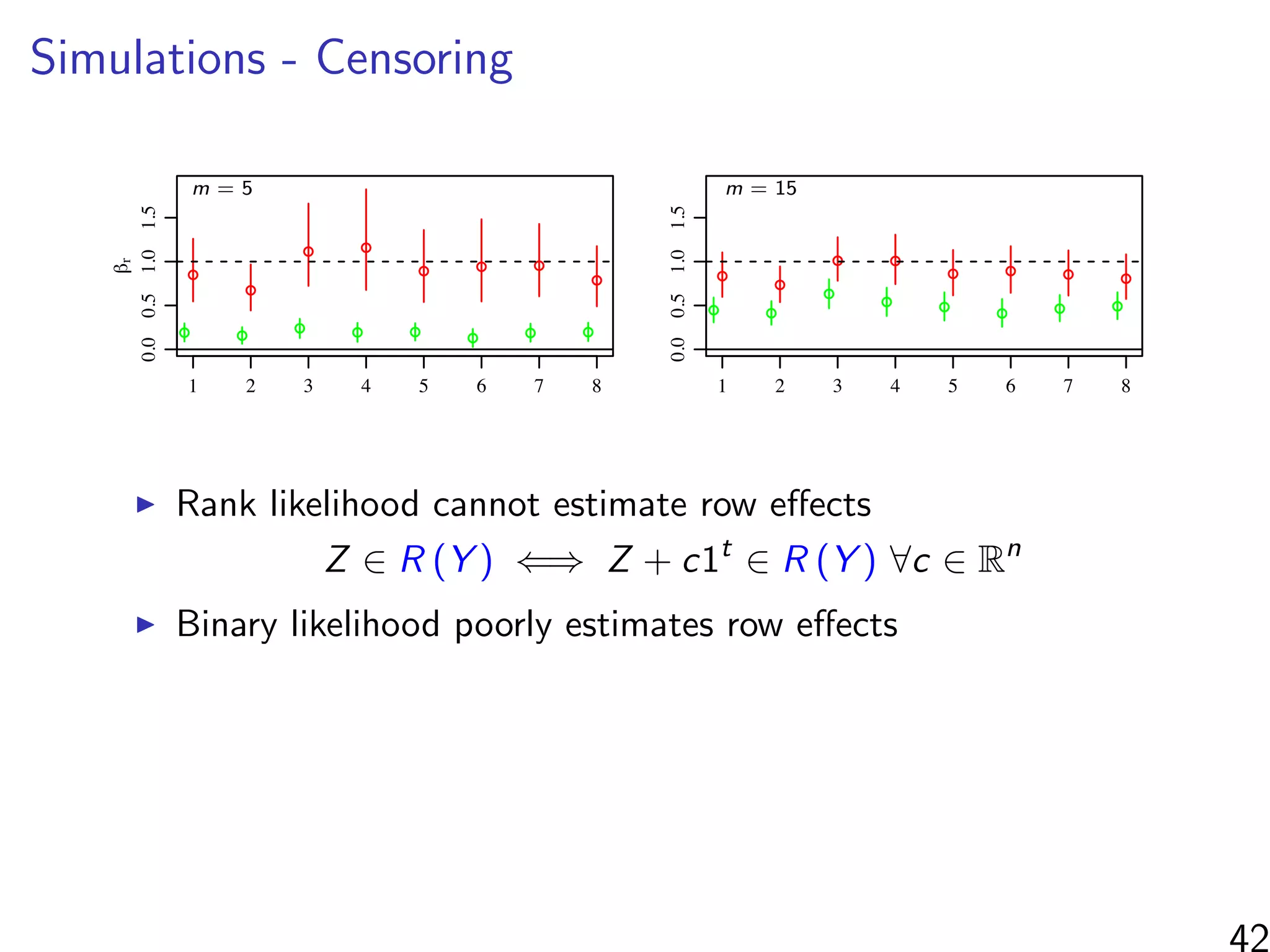
βr : row
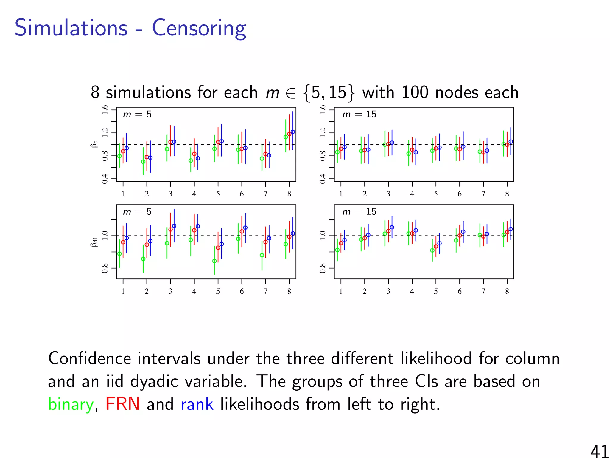
βc: column
βd1: continuous dyad
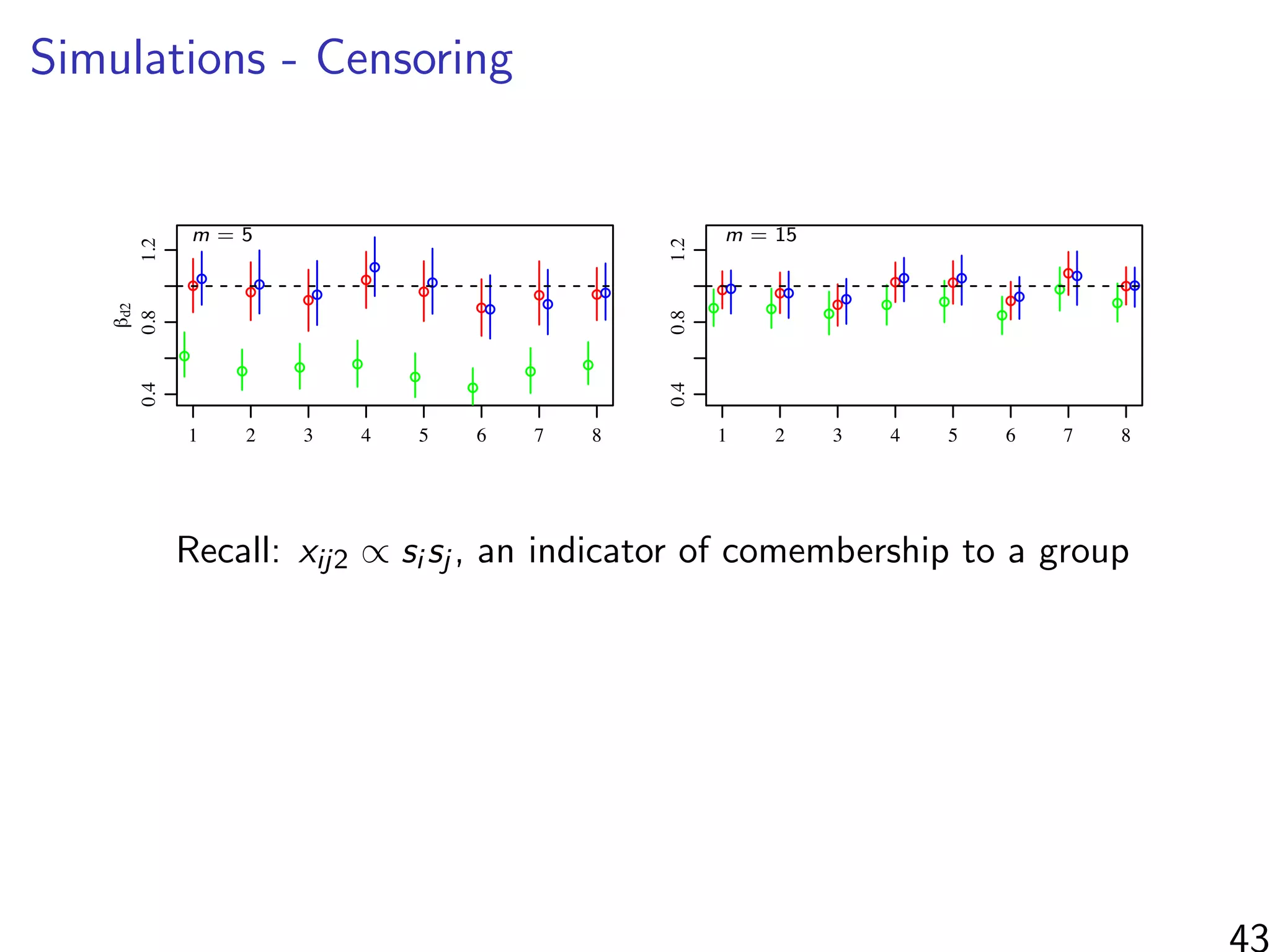
βd2: co-membership
Relative concentration around true value of each parameter:
Measured by E (β − 1)
2
|F (Y ) /E (β − 1)
2
|C (Y ) for each β
45](https://image.slidesharecdn.com/thursdaymorninglecture-latentspacemodels-170629153330/75/08-Inference-for-Networks-DYAD-Model-Overview-2017-113-2048.jpg)
![Simulations - information in the ranks
Same setup as before, but average uncensored outdegree is m
10 20 30 40 50
0.20.40.60.81.01.21.4
m
relativeconcentrationaroundtruevalue
! ! !
! !r
!
!
! ! !c
!
!
!
! !d1
! !
!
! !d2
2: Posterior concentration around true parameter values. The average of E[(β −
(S)]/E[(β − β∗)2|C(S)] across eight simulated datasets for each m ∈ {5, 15, 30, 50}.
censored binomial likelihood. As the censored binomial likelihood recognizes the censoring in
data, we expect it to provide parameter estimates that do not have the biases of the binomial
ood estimators. On the other hand, LC ignores the information in the ranks of the scored
duals, and so we might expect it to provide less precise estimates than the FRN likelihood.
βr : row
βc: column
βd1: continuous dyad
βd2: co-membership
Relative concentration around true value of each parameter:
Measured by E (β − 1)
2
|F (Y ) /E (β − 1)
2
|C (Y ) for each β
When m n, most of the information found by considering
ranked/unranked individuals as groups rather than the relative
ordering of the ranked individuals.](https://image.slidesharecdn.com/thursdaymorninglecture-latentspacemodels-170629153330/75/08-Inference-for-Networks-DYAD-Model-Overview-2017-114-2048.jpg)


![Social Network Analysis [1994]](https://cdn.slidesharecdn.com/ss_thumbnails/socialnetworkanalysis1994-160617072245-thumbnail.jpg?width=640&height=640&fit=bounds)