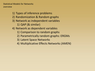
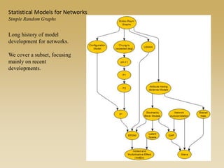
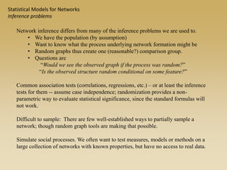
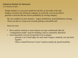
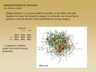
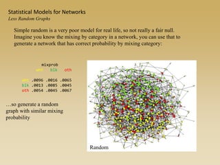
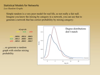
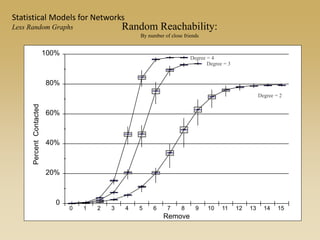
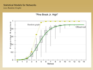
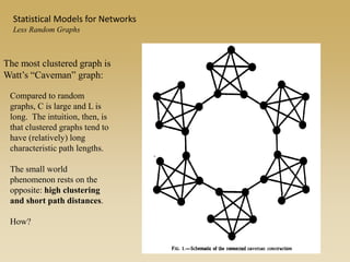
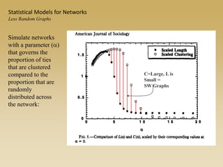
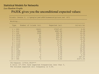
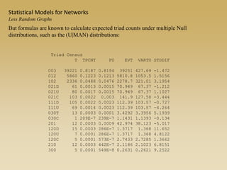
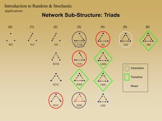
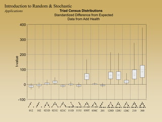
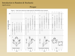
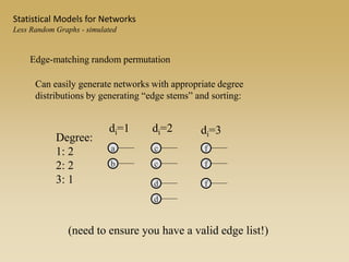
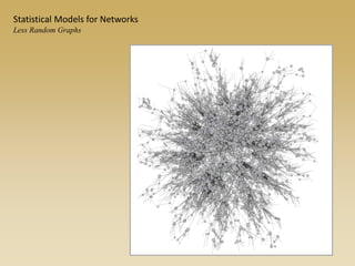
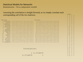
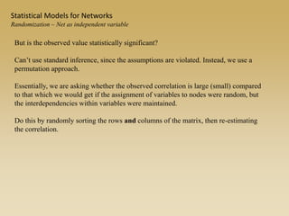
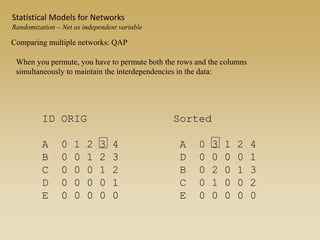
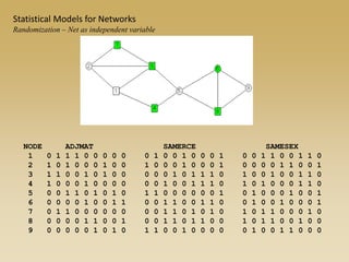
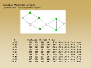
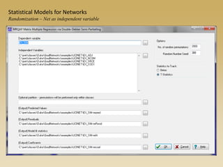
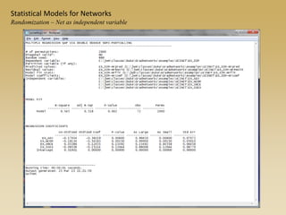
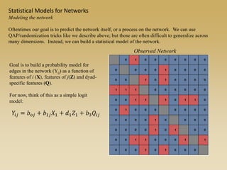
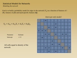
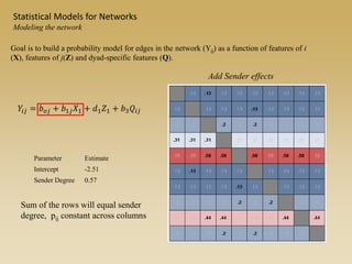
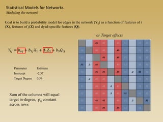
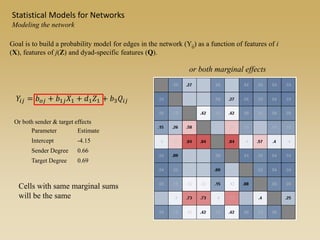
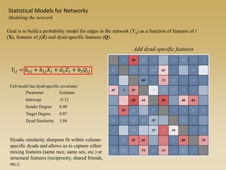
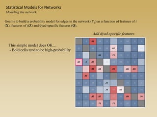
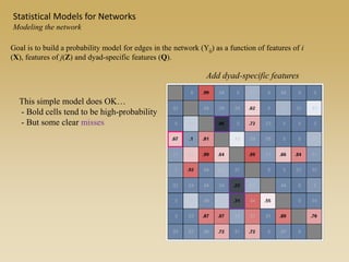
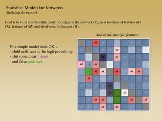
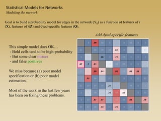
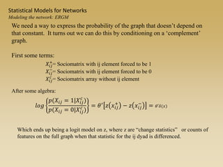
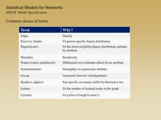
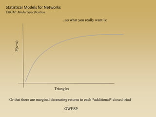
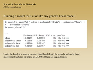
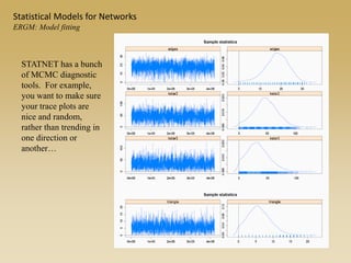
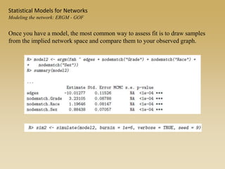
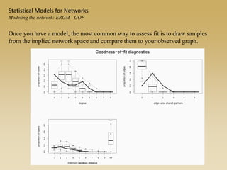
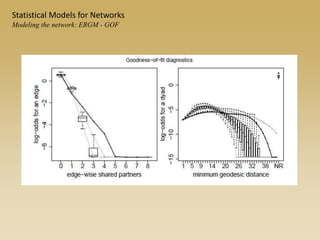
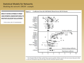
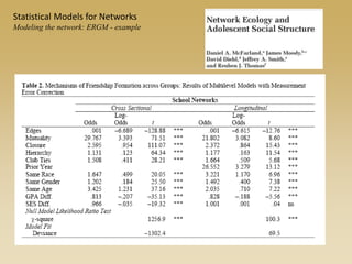
Statistical Models for Networks
https://tinyurl.com/SN-H2018
Statistical Models for Networks
overview
1) Types of inference problems
2) Randomization & Random graphs
3) Network as independent variables
1) QAP (& similar)
4) Network as dependent variables
1) Comparison to random graphs
2) Parametrically random graphs: ERGMs
3) Latent Space Networks
4) Multiplicative Effects Networks (AMEN)
Statistical Models for Networks
Simple Random Graphs
Long history of model
development for networks.
We cover a subset, focusing
mainly on recent
developments.
Network inference differs from many of the inference problems we are used to.
• We have the population (by assumption)
• Want to know what the process underlying network formation might be
• Random graphs thus create one (reasonable?) comparison group.
• Questions are
“Would we see the observed graph if the process was random?”
“Is the observed structure random conditional on some feature?”
Common association tests (correlations, regressions, etc.) – or at least the inference
tests for them -- assume case independence; randomization provides a non-
parametric way to evaluate statistical significance, since the standard formulas will
not work.
Difficult to sample: There are few well-established ways to partially sample a
network; though random graph tools are making that possible.
Simulate social processes. We often want to test measures, models or methods on a
large collection of networks with known properties, but have no access to real data.
Statistical Models for Networks
Inference problems
That is we can think of this as either a graph of n nodes and assume all edges
have equal probability of being present (G(N,p)) or we can imagine a (set of)
graph(s) chosen at random from the set of all graphs with n nodes and m edges
(G(N,M)).
Number of unique undirected graph patterns by number of nodes
But, enumeration is usually
impossible…so we use
construction rules that ensure
even probability of all graphs in
the space.
* Note a subtle difference here: the G(N,P) model will have random variability in number of edges due to random chance…ignorable in limit of
large networks.
Statistical Models for Networks
Simple random graphs
Note a core difficulty: We want to compare our observed network to the class
of all graphs (with similar properties), but we have no sampling frame of
graphs.
In a Erdos random graph - each dyad has the same probability of being tied –so algorithm is a simple
coin-flip on each dyad.
degree will be Poisson distributed, and the nodes with high degree are likely to be at the intuitive
center.
Statistical Models for Networks
Simple Random Graphs
Simple random graph with 1000 nodes and average degree=2.4  p=0.0024.
Statistical Models for Networks
Simple Random Graphs
Network connectivity
changes rapidly as a
function of network
volume.
In a Erdos-reyni
random network, when
the average degree is
<1, the network is
always disconnected.
When it is >2, there is a
“giant component” that
takes up most of the
network.
Note that this is
dependent on mean
degree, not density, so
applies to networks of
any size.
Average Degree
Statistical Models for Networks
Simple Random Graphs
Simple random is a very poor model for real life, so not really a fair null.
Imagine you know the mixing by category in a network, you can use that to
generate a network that has correct probability by mixing category:
We can condition on more features – degree distribution, dyad distribution, mixing…
These can take us a long ways towards getting a reasonable null.
Some are easy:
• Have analytic solution to some features on some conditionals (like the
“configuration model” used for building a null in community detection)
• Good algorithms exist for fixing both in & out degree
generate a set of half-edges for each node’s degree, randomly sort, put back
together
Often a tradeoff between *exact* uniform random & speed/tractabiltiy
Statistical Models for Networks
Less Random Graphs
Simple random is a very poor model for real life, so not really a fair null.
Imagine you know the mixing by category in a network, you can use that to
generate a network that has correct probability by mixing category:
mixprob
wht blk oth
wht .0096 .0016 .0065
blk .0013 .0085 .0045
oth .0054 .0045 .0067
…so generate a random
graph with similar mixing
probability
Observed
Statistical Models for Networks
Less Random Graphs
Simple random is a very poor model for real life, so not really a fair null.
Imagine you know the mixing by category in a network, you can use that to
generate a network that has correct probability by mixing category:
mixprob
wht blk oth
wht .0096 .0016 .0065
blk .0013 .0085 .0045
oth .0054 .0045 .0067
…so generate a random
graph with similar mixing
probability
Random
Statistical Models for Networks
Less Random Graphs
Simple random is a very poor model for real life, so not really a fair null.
Imagine you know the mixing by category in a network, you can use that to
generate a network that has correct probability by mixing category:
mixprob
wht blk oth
wht .0096 .0016 .0065
blk .0013 .0085 .0045
oth .0054 .0045 .0067
…so generate a random
graph with similar mixing
probability
Degree distributions
don’t match
Statistical Models for Networks
Less Random Graphs
0
20%
40%
60%
80%
100%
PercentContacted
0 1 2 3 4 5 6 7 8 9 10 11 12 13 14 15
Remove
Degree = 4
Degree = 3
Degree = 2
Random Reachability:
By number of close friends
Statistical Models for Networks
Less Random Graphs
0
0.2
0.4
0.6
0.8
1
ProportionReached
0 1 2 3 4 5 6 7 8 9 10 11 12 13 14
Remove
"Pine Brook Jr. High"
Random graph
Observed
Statistical Models for Networks
Less Random Graphs
The most clustered graph is
Watt’s “Caveman” graph:
Compared to random
graphs, C is large and L is
long. The intuition, then, is
that clustered graphs tend to
have (relatively) long
characteristic path lengths.
The small world
phenomenon rests on the
opposite: high clustering
and short path distances.
How?
Statistical Models for Networks
Less Random Graphs
C=Large, L is
Small =
SW Graphs
Simulate networks
with a parameter (a)
that governs the
proportion of ties
that are clustered
compared to the
proportion that are
randomly
distributed across
the network:
Statistical Models for Networks
Less Random Graphs
PAJEK gives you the unconditional expected values:
------------------------------------------------------------------------------
Triadic Census 2. i:peoplejwms884homeworkprison.net (67)
------------------------------------------------------------------------------
Working...
----------------------------------------------------------------------------
Type Number of triads (ni) Expected (ei) (ni-ei)/ei
----------------------------------------------------------------------------
1 - 003 39221 37227.47 0.05
2 - 012 5860 9587.83 -0.39
3 - 102 2336 205.78 10.35
4 - 021D 61 205.78 -0.70
5 - 021U 80 205.78 -0.61
6 - 021C 103 411.55 -0.75
7 - 111D 105 17.67 4.94
8 - 111U 69 17.67 2.91
9 - 030T 13 17.67 -0.26
10 - 030C 1 5.89 -0.83
11 - 201 12 0.38 30.65
12 - 120D 15 0.38 38.56
13 - 120U 7 0.38 17.46
14 - 120C 5 0.76 5.59
15 - 210 12 0.03 367.67
16 - 300 5 0.00 21471.04
----------------------------------------------------------------------------
Chi-Square: 137414.3919***
6 cells (37.50%) have expected frequencies less than 5.
The minimum expected cell frequency is 0.00.
Statistical Models for Networks
Less Random Graphs
But formulas are known to calculate expected triad counts under multiple Null
distributions, such as the (U|MAN) distributions:
Triad Census
T TPCNT PU EVT VARTU STDDIF
003 39221 0.8187 0.8194 39251 427.69 -1.472
012 5860 0.1223 0.1213 5810.8 1053.5 1.5156
102 2336 0.0488 0.0476 2278.7 321.01 3.1954
021D 61 0.0013 0.0015 70.949 67.37 -1.212
021U 80 0.0017 0.0015 70.949 67.37 1.1027
021C 103 0.0022 0.003 141.9 127.58 -3.444
111D 105 0.0022 0.0023 112.39 103.57 -0.727
111U 69 0.0014 0.0023 112.39 103.57 -4.264
030T 13 0.0003 0.0001 3.4292 3.3956 5.1939
030C 1 209E-7 239E-7 1.1431 1.1393 -0.134
201 12 0.0003 0.0009 42.974 38.123 -5.017
120D 15 0.0003 286E-7 1.3717 1.368 11.652
120U 7 0.0001 286E-7 1.3717 1.368 4.8122
120C 5 0.0001 573E-7 2.7433 2.7285 1.3662
210 12 0.0003 442E-7 2.1186 2.1023 6.8151
300 5 0.0001 549E-8 0.2631 0.2621 9.2522
Statistical Models for Networks
Less Random Graphs
Network Sub-Structure: Triads
003
(0)
012
(1)
102
021D
021U
021C
(2)
111D
111U
030T
030C
(3)
201
120D
120U
120C
(4)
210
(5)
300
(6)
Intransitive
Transitive
Mixed
Introduction to Random & Stochastic
Applications
-100
0
100
200
300
400
t-value
Triad Census Distributions
Standardized Difference from Expected
Data from Add Health
012 102 021D 021U 021C 111D 111U 030T 030C 201 120D 120U 120C 210 300
Introduction to Random & Stochastic
Applications
Prosper
Introduction to Random & Stochastic
Applications
Edge-matching random permutation
Can easily generate networks with appropriate degree
distributions by generating “edge stems” and sorting:
a
Degree:
1: 2
2: 2
3: 1
b
di=1
c
c
di=2
d
d
f
f
di=3
f
(need to ensure you have a valid edge list!)
Statistical Models for Networks
Less Random Graphs - simulated
Statistical Models for Networks
Less Random Graphs
Statistical Models for Networks
Less Random Graphs
So the answer to the inference problem is to construct a reasonable approximation to
your observed setting (or social process) and compare.
There are many ways to conceive of “reasonable” and many ways to construct each.
When possible, use analytic solutions; but that’s rarely possible for realistic
comparisons.
Comparing multiple networks: QAP
The substantive question is how one set of relations (or dyadic attributes) relates to
another.
For example:
• Do marriage ties correlate with business ties in the Medici family network?
• Are friendship relations correlated with joint membership in a club?
Statistical Models for Networks
Randomization – Net as independent variable
Assessing the correlation is straight forward, as we simply correlate each
corresponding cell of the two matrices:
Marriage
1 ACCIAIUOL 0 0 0 0 0 0 0 0 1 0 0 0 0 0 0 0
2 ALBIZZI 0 0 0 0 0 1 1 0 1 0 0 0 0 0 0 0
3 BARBADORI 0 0 0 0 1 0 0 0 1 0 0 0 0 0 0 0
4 BISCHERI 0 0 0 0 0 0 1 0 0 0 1 0 0 0 1 0
5 CASTELLAN 0 0 1 0 0 0 0 0 0 0 1 0 0 0 1 0
6 GINORI 0 1 0 0 0 0 0 0 0 0 0 0 0 0 0 0
7 GUADAGNI 0 1 0 1 0 0 0 1 0 0 0 0 0 0 0 1
8 LAMBERTES 0 0 0 0 0 0 1 0 0 0 0 0 0 0 0 0
9 MEDICI 1 1 1 0 0 0 0 0 0 0 0 0 1 1 0 1
10 PAZZI 0 0 0 0 0 0 0 0 0 0 0 0 0 1 0 0
11 PERUZZI 0 0 0 1 1 0 0 0 0 0 0 0 0 0 1 0
12 PUCCI 0 0 0 0 0 0 0 0 0 0 0 0 0 0 0 0
13 RIDOLFI 0 0 0 0 0 0 0 0 1 0 0 0 0 0 1 1
14 SALVIATI 0 0 0 0 0 0 0 0 1 1 0 0 0 0 0 0
15 STROZZI 0 0 0 1 1 0 0 0 0 0 1 0 1 0 0 0
16 TORNABUON 0 0 0 0 0 0 1 0 1 0 0 0 1 0 0 0
Business
1 0 0 0 0 0 0 0 0 0 0 0 0 0 0 0 0
2 0 0 0 0 0 0 0 0 0 0 0 0 0 0 0 0
3 0 0 0 0 1 1 0 0 1 0 1 0 0 0 0 0
4 0 0 0 0 0 0 1 1 0 0 1 0 0 0 0 0
5 0 0 1 0 0 0 0 1 0 0 1 0 0 0 0 0
6 0 0 1 0 0 0 0 0 1 0 0 0 0 0 0 0
7 0 0 0 1 0 0 0 1 0 0 0 0 0 0 0 0
8 0 0 0 1 1 0 1 0 0 0 1 0 0 0 0 0
9 0 0 1 0 0 1 0 0 0 1 0 0 0 1 0 1
10 0 0 0 0 0 0 0 0 1 0 0 0 0 0 0 0
11 0 0 1 1 1 0 0 1 0 0 0 0 0 0 0 0
12 0 0 0 0 0 0 0 0 0 0 0 0 0 0 0 0
13 0 0 0 0 0 0 0 0 0 0 0 0 0 0 0 0
14 0 0 0 0 0 0 0 0 1 0 0 0 0 0 0 0
15 0 0 0 0 0 0 0 0 0 0 0 0 0 0 0 0
16 0 0 0 0 0 0 0 0 1 0 0 0 0 0 0 0
Dyads:
1 2 0 0
1 3 0 0
1 4 0 0
1 5 0 0
1 6 0 0
1 7 0 0
1 8 0 0
1 9 1 0
1 10 0 0
1 11 0 0
1 12 0 0
1 13 0 0
1 14 0 0
1 15 0 0
1 16 0 0
2 1 0 0
2 3 0 0
2 4 0 0
2 5 0 0
2 6 1 0
2 7 1 0
2 8 0 0
2 9 1 0
2 10 0 0
2 11 0 0
2 12 0 0
2 13 0 0
2 14 0 0
2 15 0 0
2 16 0 0
Correlation:
1 0.3718679
0.3718679 1
Statistical Models for Networks
Randomization – Net as independent variable
But is the observed value statistically significant?
Can’t use standard inference, since the assumptions are violated. Instead, we use a
permutation approach.
Essentially, we are asking whether the observed correlation is large (small) compared
to that which we would get if the assignment of variables to nodes were random, but
the interdependencies within variables were maintained.
Do this by randomly sorting the rows and columns of the matrix, then re-estimating
the correlation.
Statistical Models for Networks
Randomization – Net as independent variable
Comparing multiple networks: QAP
When you permute, you have to permute both the rows and the columns
simultaneously to maintain the interdependencies in the data:
ID ORIG
A 0 1 2 3 4
B 0 0 1 2 3
C 0 0 0 1 2
D 0 0 0 0 1
E 0 0 0 0 0
Sorted
A 0 3 1 2 4
D 0 0 0 0 1
B 0 2 0 1 3
C 0 1 0 0 2
E 0 0 0 0 0
Statistical Models for Networks
Randomization – Net as independent variable
Procedure:
1. Calculate the observed correlation
2. for K iterations do:
a) randomly sort one of the matrices
b) recalculate the correlation
c) store the outcome
3. compare the observed correlation to the distribution of
correlations created by the random permutations.
Statistical Models for Networks
Randomization – Net as independent variable
Statistical Models for Networks
Randomization – Net as independent variable
QAP MATRIX CORRELATION
--------------------------------------------------------------------------------
Observed matrix: PadgBUS
Structure matrix: PadgMAR
# of Permutations: 2500
Random seed: 356
Univariate statistics
1 2
PadgBUS PadgMAR
------- -------
1 Mean 0.125 0.167
2 Std Dev 0.331 0.373
3 Sum 30.000 40.000
4 Variance 0.109 0.139
5 SSQ 30.000 40.000
6 MCSSQ 26.250 33.333
7 Euc Norm 5.477 6.325
8 Minimum 0.000 0.000
9 Maximum 1.000 1.000
10 N of Obs 240.000 240.000
Hubert's gamma: 16.000
Bivariate Statistics
1 2 3 4 5 6 7
Value Signif Avg SD P(Large) P(Small) NPerm
--------- --------- --------- --------- --------- --------- ---------
1 Pearson Correlation: 0.372 0.000 0.001 0.092 0.000 1.000 2500.000
2 Simple Matching: 0.842 0.000 0.750 0.027 0.000 1.000 2500.000
3 Jaccard Coefficient: 0.296 0.000 0.079 0.046 0.000 1.000 2500.000
4 Goodman-Kruskal Gamma: 0.797 0.000 -0.064 0.382 0.000 1.000 2500.000
5 Hamming Distance: 38.000 0.000 59.908 5.581 1.000 0.000 2500.000
This can be done
simply in UCINET & R
Using the same logic,we can estimate alternative models, such as
regression, logits, probits, etc. Only complication is that you need
to permute all of the independent matrices in the same way each
iteration.
Statistical Models for Networks
Randomization – Net as independent variable
NODE ADJMAT SAMERCE SAMESEX
1 0 1 1 1 0 0 0 0 0 0 1 0 0 1 0 0 0 1 0 0 1 1 0 0 1 1 0
2 1 0 1 0 0 0 1 0 0 1 0 0 0 1 0 0 0 1 0 0 0 0 1 1 0 0 1
3 1 1 0 0 1 0 1 0 0 0 0 0 1 0 1 1 1 0 1 0 0 1 0 0 1 1 0
4 1 0 0 0 1 0 0 0 0 0 0 1 0 0 1 1 1 0 1 0 1 0 0 0 1 1 0
5 0 0 1 1 0 1 0 1 0 1 1 0 0 0 0 0 0 1 0 1 0 0 0 1 0 0 1
6 0 0 0 0 1 0 0 1 1 0 0 1 1 0 0 1 1 0 0 1 0 0 1 0 0 0 1
7 0 1 1 0 0 0 0 0 0 0 0 1 1 0 1 0 1 0 1 0 1 1 0 0 0 1 0
8 0 0 0 0 1 1 0 0 1 0 0 1 1 0 1 1 0 0 1 0 1 1 0 0 1 0 0
9 0 0 0 0 0 1 0 1 0 1 1 0 0 1 0 0 0 0 0 1 0 0 1 1 0 0 0
Statistical Models for Networks
Randomization – Net as independent variable
Distance (Dij=abs(Yi-Yj)
.000 .277 .228 .181 .278 .298 .095 .307 .481
.277 .000 .049 .096 .555 .575 .182 .584 .758
.228 .049 .000 .047 .506 .526 .134 .535 .710
.181 .096 .047 .000 .459 .479 .087 .488 .663
.278 .555 .506 .459 .000 .020 .372 .029 .204
.298 .575 .526 .479 .020 .000 .392 .009 .184
.095 .182 .134 .087 .372 .392 .000 .401 .576
.307 .584 .535 .488 .029 .009 .401 .000 .175
.481 .758 .710 .663 .204 .184 .576 .175 .000
Y
0.32
0.59
0.54
0.50
0.04
0.02
0.41
0.01
-0.17
Statistical Models for Networks
Randomization – Net as independent variable
Statistical Models for Networks
Randomization – Net as independent variable
Statistical Models for Networks
Randomization – Net as independent variable
Statistical Models for Networks
Randomization – Net as independent variable
Statistical Models for Networks
Modeling the network
Oftentimes our goal is to predict the network itself, or a process on the network. We can use
QAP/randomization tricks like we describe above; but those are often difficult to generalize across
many dimensions. Instead, we can build a statistical model of the network.
𝑌𝑖𝑗 = 𝑏 𝑜𝑗 + 𝑏1𝑗 𝑋1 + 𝑑1 𝑍1 + 𝑏3 𝑄𝑖𝑗
Goal is to build a probability model for
edges in the network (Yij) as a function of
features of i (X), features of j(Z) and dyad-
specific features (Q).
For now, think of this as a simple logit
model:
Observed Network
Intercept only model:
Goal is to build a probability model for edges in the network (Yij) as a function of features of i
(X), features of j(Z) and dyad-specific features (Q).
𝑌𝑖𝑗 = 𝑏 𝑜𝑗 + 𝑏1𝑗 𝑋1 + 𝑑1 𝑍1 + 𝑏3 𝑄𝑖𝑗
Parameter Estimate
Intercept -1.13
All cells equal to density of the
network
Statistical Models for Networks
Modeling the network
𝑌𝑖𝑗 = 𝑏 𝑜𝑗 + 𝑏1𝑗 𝑋1 + 𝑑1 𝑍1 + 𝑏3 𝑄𝑖𝑗
Add Sender effects
Parameter Estimate
Intercept -2.51
Sender Degree 0.57
Sum of the rows will equal sender
degree, pij constant across columns
Goal is to build a probability model for edges in the network (Yij) as a function of features of i
(X), features of j(Z) and dyad-specific features (Q).
Statistical Models for Networks
Modeling the network
𝑌𝑖𝑗 = 𝑏 𝑜𝑗 + 𝑏1𝑗 𝑋1 + 𝑑1 𝑍1 + 𝑏3 𝑄𝑖𝑗
Parameter Estimate
Intercept -2.57
Target Degree 0.59
Sum of the columns will equal
target in-degree, pij constant
across rows
or Target effects
Goal is to build a probability model for edges in the network (Yij) as a function of features of i
(X), features of j(Z) and dyad-specific features (Q).
Statistical Models for Networks
Modeling the network
𝑌𝑖𝑗 = 𝑏 𝑜𝑗 + 𝑏1𝑗 𝑋1 + 𝑑1 𝑍1 + 𝑏3 𝑄𝑖𝑗
Or both sender & target effects
Parameter Estimate
Intercept -4.15
Sender Degree 0.66
Target Degree 0.69
Cells with same marginal sums
will be the same
or both marginal effects
Goal is to build a probability model for edges in the network (Yij) as a function of features of i
(X), features of j(Z) and dyad-specific features (Q).
Statistical Models for Networks
Modeling the network
𝑌𝑖𝑗 = 𝑏 𝑜𝑗 + 𝑏1𝑗 𝑋1 + 𝑑1 𝑍1 + 𝑏3 𝑄𝑖𝑗
Full model has dyad-specific covariates
Parameter Estimate
Intercept -9.12
Sender Degree 0.49
Target Degree 0.87
Dyad Similarity 1.86
Dyadic similarity sharpens fit within volume-
specific dyads and allows us to capture either
mixing features (same race, same sex, etc.) or
structural features (reciprocity, shared friends,
etc.).
Add dyad-specific features
Goal is to build a probability model for edges in the network (Yij) as a function of features of i
(X), features of j(Z) and dyad-specific features (Q).
Statistical Models for Networks
Modeling the network
Add dyad-specific features
Goal is to build a probability model for edges in the network (Yij) as a function of features of i
(X), features of j(Z) and dyad-specific features (Q).
Statistical Models for Networks
Modeling the network
This simple model does OK…
- Bold cells tend to be high-probability
- But some clear misses
- and false positives
We miss because (a) poor model
specification or (b) poor model
estimation.
Most of the work in the last few years
has been on fixing these problems.
A key twist on this simple model above is that while we work with dyads (i.e.
our observations in the dataset will be ij dyads), the model is of the entire
network – including all the dependencies.
Substantively, the approach is to ask whether the graph in question is an element
of the class of all random graphs with the given known elements. For example,
all graphs with 5 nodes and 3 edges, or, put probabilistically, the probability of
observing the current graph given the conditions.
Statistical Models for Networks
Modeling the network: ERGM
The “p1” model of Holland and Leinhardt is the classic foundation
– the basic idea is that you can generate a statistical model of the
network by predicting the counts of types of ties (asym, null, sym).
They formulate a log-linear model for these counts; but the model
is equivalent to a logit model on the dyads:
Note the subscripts! This implies a distinct parameter for every
node i and j in the model, plus one for reciprocity.
Statistical Models for Networks
Modeling the network: ERGM
𝑙𝑜𝑔𝑖𝑡 𝑋𝑖𝑗 = 1 = 𝛼𝑖 + 𝛽𝑗 + 𝜌(𝑋𝑖𝑗)
Statistical Models for Networks
Modeling the network: ERGM
Results from SAS version on PROSPER datasets
Statistical Models for Networks
Modeling the network: ERGM
Once you know the basic model format, you can imagine other
specifications:
Key is to ensure that the specification doesn’t imply a linear
dependency of terms.
Model fit is hard to judge, and for all but the simplest rhs features,
the se’s are “approximate.”
How to fix the inference problem?
Logit 𝑋𝑖𝑗 = 1 = 𝛼𝑖 + 𝛽𝑗 + 𝜌(𝑋𝑖𝑗)
Logit 𝑋𝑖𝑗 = 1 = 𝛼𝑖 + 𝛽𝑗 + 𝜌 𝑔(𝑋𝑖𝑗) – differential reciprocity
Logit 𝑋𝑖𝑗 = 1 = 𝛼𝑖 + 𝛽𝑗 + 𝜌 𝑔(𝑋𝑖𝑗) + (node attributes)
Statistical Models for Networks
Modeling the network: ERGM
Where:
q is a vector of parameters (like regression coefficients)
z is a vector of network statistics, conditioning the graph
k is a normalizing constant, to ensure the probabilities sum to 1.
𝑝 𝑋 = 𝑥 =
𝑒𝑥𝑝 𝜃′
𝑧 𝑥
𝑘 𝜃
Statistical Models for Networks
Modeling the network: ERGM
Analytic & estimation solutions came with some careful thinking on the underlying
structure on this model. Start with a re-expression of a general graph model:
So here, we’re just asking the probability of observing our network, given some network
statistics.
We need a way to express the probability of the graph that doesn’t depend on
that constant. It turns out we can do this by conditioning on a ‘complement’
graph.
First some terms:
𝑋𝑖𝑗
+
= Sociomatrix with ij element forced to be 1
𝑋𝑖𝑗
−
= Sociomatrix with ij element forced to be 0
𝑋𝑖𝑗
𝑐
= Sociomatrix array without ij element
𝑙𝑜𝑔
𝑝(𝑋𝑖𝑗 = 1|𝑋𝑖𝑗
𝑐
)
𝑝(𝑋𝑖𝑗 = 0|𝑋𝑖𝑗
𝑐
)
= 𝜃′ 𝑧 𝑥𝑖𝑗
+
− 𝑧 𝑥𝑖𝑗
−
= 𝜃′𝛿(𝑥)
After some algebra:
Which ends up being a logit model on z, where z are “change statistics” or counts of
features on the full graph when that statistic for the ij dyad is differenced.
Statistical Models for Networks
Modeling the network: ERGM
Statistical Models for Networks
Modeling the network: ERGM
Steps in estimating an ERGM
1) Specify the model
2) Fit the model
3) Examine MCMC chains for convergence & such
4) Examine Goodness of fit
1) If poor, return to 1
2) Else, publish your paper. 
Question is the
likelihood of a network
given an observed set of
network mixing
statistics.
The set of such statistics
(“terms”) is large…and
growing.
Intuitively, these capture
a social process you
think is driving network
formation.
Statistical Models for Networks
ERGM: Model Specification
Theory
Small-Worlds
Preferential
Attachment
Homophily
Social Balance
Birds of a feather…
Colloquialism
Structural
Signature Model Term
A friend of a friend...
A friend of an enemy…
Don’t I know your…
or
Kevin Bacon game…
Rich get richer..
First mover advantage
NodeMatch()
Balance,
Transitivity,
GWESP
Clustering & k-
paths
In-degree, k-stars
Statistical Models for Networks
ERGM: Model Specification
Common classes of terms:
Term Why?
Edges Density
Receiver, Sender Fit person specific degree distribution
Degree(d,attr) Fit the observed global degree distribution, perhaps
by attribute
Mutuality Reciprocity
Nodecov(attr), nodefactor() Differential row/colloumn effects by an attribute
Nodematch(attr) Homophily on a particular attribute
Gwesp Geometric form for closed partners
Dyadcov, edgecov Pair specific covariates, differ by directed or not.
Isolates Fit the number of isolated nodes in the graph
Cycle(k) Fit cycles of length k (slow!)
Statistical Models for Networks
ERGM: Model Specification
Model Sensitivity
ERGM models are very sensitive to model specification, and work best if
you have a good intuition about how the interdependencies in a network
operate – most of us do not have that intuition!
Model Degeneracy: Intuitively, it happens when the network
sample space implied by the model does not contain any instances
of your model.
Example: Simple model of edges & triangles.
Intuitively, we’d expect from balance a positive coefficient on
triangles.
Statistical Models for Networks
ERGM: Model Specification
Statistical Models for Networks
ERGM: Model Specification
Triangles
Intuition from regression: b(triangle) is positive
P(x=x)
Statistical Models for Networks
ERGM: Model Specification
But note the model really says “more closed triads is good”
So if this is good… ..this is better!
Statistical Models for Networks
ERGM: Model Specification
Triangles
..so what you really want is:
P(x=x)
Or that there are marginal decreasing returns to each *additional* closed triad
GWESP
Running a model feels a lot like any general linear model:
Statistical Models for Networks
ERGM: Model fitting
Under the hood, it’s using a pseudo-=likelihood (logit) for models with only dyad-
independent features, or fitting an MCMC if there are dependencies.
Statistical Models for Networks
ERGM: Model fitting
STATNET has a bunch
of MCMC diagnostic
tools. For example,
you want to make sure
your trace plots are
nice and random,
rather than trending in
one direction or
another…
Once you have a model, the most common way to assess fit is to draw samples
from the implied network space and compare them to your observed graph.
Statistical Models for Networks
Modeling the network: ERGM - GOF
Once you have a model, the most common way to assess fit is to draw samples
from the implied network space and compare them to your observed graph.
Statistical Models for Networks
Modeling the network: ERGM - GOF
Statistical Models for Networks
Modeling the network: ERGM - GOF
Statistical Models for Networks
Modeling the network: ERGM - example
Statistical Models for Networks
Modeling the network: ERGM - example
Statistical Models for Networks
Modeling the network: ERGM - example
Introduction to Random & Stochastic
Latent Space Models
Introduction to Random & Stochastic
Latent Space Models
Simple latent distance model:
Given a distribution of points in the space defined by z, probability of a tie
decreases with their distance in the latent space.
Z can be as many dimensions as you want; typically we try to fit the minimum
number of dimensions that provide reasonable fit to the data.
Introduction to Random & Stochastic
Latent Space Models
2d solution
for Sampson
monistary
data
Z = a dimension in some unknown
space that, once accounted for makes
ties independent.
In addition, we can now embed z
within a group structure, which adds
probability of ingroup ties.
Introduction to Random & Stochastic
Latent Space Models: with groups
Introduction to Random & Stochastic
Latent Space Models
Example with the
Prosper data, with
three groups
Introduction to Random & Stochastic
Latent Space Models
Introduction to Random & Stochastic
Latent Space Models
Latent space models tend to be (a) much more robust to model specification errors
than are ERGMs and (b) have better known convergance properties (i.e. you can
prove that the models will converge, which follows because you’re making a
conditional independence assumption that’s not made in ERGM).
But, you rarely know what the dimensions mean socially. So it provides a fit, but
doesn’t test a mechanism.
This is a key difference; if you’re goal is out of sample prediction or simply
controlling the “noise” of a network, a latent space model is probably the best
solution. If your goal is to test a particular network mechanism, an ERGM is
probably better.
Introduction to Random & Stochastic
Generalizations
AMEN: Additive & multiplicative effects models (Hoff & Volfovsky)
Basic social relations model
Dyad
effects
Row
effects
Column
effects
Row
error
Col
error
dyad
error
More general frame:
Latent
multiplicative
covariance
Model is very general; can deal with y on any scale (binary to real
values), fits latent space & observed covariates.
Computationally intensive…
Introduction to Random & Stochastic
Generalizations
For more detail, see last
year’s presentation by
Alex!
08 Statistical Models for Nets I, cross-section

08 Statistical Models for Nets I, cross-section

  • 1.
    Statistical Models forNetworks https://tinyurl.com/SN-H2018
  • 2.
    Statistical Models forNetworks overview 1) Types of inference problems 2) Randomization & Random graphs 3) Network as independent variables 1) QAP (& similar) 4) Network as dependent variables 1) Comparison to random graphs 2) Parametrically random graphs: ERGMs 3) Latent Space Networks 4) Multiplicative Effects Networks (AMEN)
  • 3.
    Statistical Models forNetworks Simple Random Graphs Long history of model development for networks. We cover a subset, focusing mainly on recent developments.
  • 4.
    Network inference differsfrom many of the inference problems we are used to. • We have the population (by assumption) • Want to know what the process underlying network formation might be • Random graphs thus create one (reasonable?) comparison group. • Questions are “Would we see the observed graph if the process was random?” “Is the observed structure random conditional on some feature?” Common association tests (correlations, regressions, etc.) – or at least the inference tests for them -- assume case independence; randomization provides a non- parametric way to evaluate statistical significance, since the standard formulas will not work. Difficult to sample: There are few well-established ways to partially sample a network; though random graph tools are making that possible. Simulate social processes. We often want to test measures, models or methods on a large collection of networks with known properties, but have no access to real data. Statistical Models for Networks Inference problems
  • 5.
    That is wecan think of this as either a graph of n nodes and assume all edges have equal probability of being present (G(N,p)) or we can imagine a (set of) graph(s) chosen at random from the set of all graphs with n nodes and m edges (G(N,M)). Number of unique undirected graph patterns by number of nodes But, enumeration is usually impossible…so we use construction rules that ensure even probability of all graphs in the space. * Note a subtle difference here: the G(N,P) model will have random variability in number of edges due to random chance…ignorable in limit of large networks. Statistical Models for Networks Simple random graphs Note a core difficulty: We want to compare our observed network to the class of all graphs (with similar properties), but we have no sampling frame of graphs.
  • 6.
    In a Erdosrandom graph - each dyad has the same probability of being tied –so algorithm is a simple coin-flip on each dyad. degree will be Poisson distributed, and the nodes with high degree are likely to be at the intuitive center. Statistical Models for Networks Simple Random Graphs
  • 7.
    Simple random graphwith 1000 nodes and average degree=2.4  p=0.0024. Statistical Models for Networks Simple Random Graphs
  • 8.
    Network connectivity changes rapidlyas a function of network volume. In a Erdos-reyni random network, when the average degree is <1, the network is always disconnected. When it is >2, there is a “giant component” that takes up most of the network. Note that this is dependent on mean degree, not density, so applies to networks of any size. Average Degree Statistical Models for Networks Simple Random Graphs
  • 9.
    Simple random isa very poor model for real life, so not really a fair null. Imagine you know the mixing by category in a network, you can use that to generate a network that has correct probability by mixing category: We can condition on more features – degree distribution, dyad distribution, mixing… These can take us a long ways towards getting a reasonable null. Some are easy: • Have analytic solution to some features on some conditionals (like the “configuration model” used for building a null in community detection) • Good algorithms exist for fixing both in & out degree generate a set of half-edges for each node’s degree, randomly sort, put back together Often a tradeoff between *exact* uniform random & speed/tractabiltiy Statistical Models for Networks Less Random Graphs
  • 10.
    Simple random isa very poor model for real life, so not really a fair null. Imagine you know the mixing by category in a network, you can use that to generate a network that has correct probability by mixing category: mixprob wht blk oth wht .0096 .0016 .0065 blk .0013 .0085 .0045 oth .0054 .0045 .0067 …so generate a random graph with similar mixing probability Observed Statistical Models for Networks Less Random Graphs
  • 11.
    Simple random isa very poor model for real life, so not really a fair null. Imagine you know the mixing by category in a network, you can use that to generate a network that has correct probability by mixing category: mixprob wht blk oth wht .0096 .0016 .0065 blk .0013 .0085 .0045 oth .0054 .0045 .0067 …so generate a random graph with similar mixing probability Random Statistical Models for Networks Less Random Graphs
  • 12.
    Simple random isa very poor model for real life, so not really a fair null. Imagine you know the mixing by category in a network, you can use that to generate a network that has correct probability by mixing category: mixprob wht blk oth wht .0096 .0016 .0065 blk .0013 .0085 .0045 oth .0054 .0045 .0067 …so generate a random graph with similar mixing probability Degree distributions don’t match Statistical Models for Networks Less Random Graphs
  • 13.
    0 20% 40% 60% 80% 100% PercentContacted 0 1 23 4 5 6 7 8 9 10 11 12 13 14 15 Remove Degree = 4 Degree = 3 Degree = 2 Random Reachability: By number of close friends Statistical Models for Networks Less Random Graphs
  • 14.
    0 0.2 0.4 0.6 0.8 1 ProportionReached 0 1 23 4 5 6 7 8 9 10 11 12 13 14 Remove "Pine Brook Jr. High" Random graph Observed Statistical Models for Networks Less Random Graphs
  • 15.
    The most clusteredgraph is Watt’s “Caveman” graph: Compared to random graphs, C is large and L is long. The intuition, then, is that clustered graphs tend to have (relatively) long characteristic path lengths. The small world phenomenon rests on the opposite: high clustering and short path distances. How? Statistical Models for Networks Less Random Graphs
  • 16.
    C=Large, L is Small= SW Graphs Simulate networks with a parameter (a) that governs the proportion of ties that are clustered compared to the proportion that are randomly distributed across the network: Statistical Models for Networks Less Random Graphs
  • 17.
    PAJEK gives youthe unconditional expected values: ------------------------------------------------------------------------------ Triadic Census 2. i:peoplejwms884homeworkprison.net (67) ------------------------------------------------------------------------------ Working... ---------------------------------------------------------------------------- Type Number of triads (ni) Expected (ei) (ni-ei)/ei ---------------------------------------------------------------------------- 1 - 003 39221 37227.47 0.05 2 - 012 5860 9587.83 -0.39 3 - 102 2336 205.78 10.35 4 - 021D 61 205.78 -0.70 5 - 021U 80 205.78 -0.61 6 - 021C 103 411.55 -0.75 7 - 111D 105 17.67 4.94 8 - 111U 69 17.67 2.91 9 - 030T 13 17.67 -0.26 10 - 030C 1 5.89 -0.83 11 - 201 12 0.38 30.65 12 - 120D 15 0.38 38.56 13 - 120U 7 0.38 17.46 14 - 120C 5 0.76 5.59 15 - 210 12 0.03 367.67 16 - 300 5 0.00 21471.04 ---------------------------------------------------------------------------- Chi-Square: 137414.3919*** 6 cells (37.50%) have expected frequencies less than 5. The minimum expected cell frequency is 0.00. Statistical Models for Networks Less Random Graphs
  • 18.
    But formulas areknown to calculate expected triad counts under multiple Null distributions, such as the (U|MAN) distributions: Triad Census T TPCNT PU EVT VARTU STDDIF 003 39221 0.8187 0.8194 39251 427.69 -1.472 012 5860 0.1223 0.1213 5810.8 1053.5 1.5156 102 2336 0.0488 0.0476 2278.7 321.01 3.1954 021D 61 0.0013 0.0015 70.949 67.37 -1.212 021U 80 0.0017 0.0015 70.949 67.37 1.1027 021C 103 0.0022 0.003 141.9 127.58 -3.444 111D 105 0.0022 0.0023 112.39 103.57 -0.727 111U 69 0.0014 0.0023 112.39 103.57 -4.264 030T 13 0.0003 0.0001 3.4292 3.3956 5.1939 030C 1 209E-7 239E-7 1.1431 1.1393 -0.134 201 12 0.0003 0.0009 42.974 38.123 -5.017 120D 15 0.0003 286E-7 1.3717 1.368 11.652 120U 7 0.0001 286E-7 1.3717 1.368 4.8122 120C 5 0.0001 573E-7 2.7433 2.7285 1.3662 210 12 0.0003 442E-7 2.1186 2.1023 6.8151 300 5 0.0001 549E-8 0.2631 0.2621 9.2522 Statistical Models for Networks Less Random Graphs
  • 19.
  • 20.
    -100 0 100 200 300 400 t-value Triad Census Distributions StandardizedDifference from Expected Data from Add Health 012 102 021D 021U 021C 111D 111U 030T 030C 201 120D 120U 120C 210 300 Introduction to Random & Stochastic Applications
  • 21.
    Prosper Introduction to Random& Stochastic Applications
  • 22.
    Edge-matching random permutation Caneasily generate networks with appropriate degree distributions by generating “edge stems” and sorting: a Degree: 1: 2 2: 2 3: 1 b di=1 c c di=2 d d f f di=3 f (need to ensure you have a valid edge list!) Statistical Models for Networks Less Random Graphs - simulated
  • 23.
    Statistical Models forNetworks Less Random Graphs
  • 24.
    Statistical Models forNetworks Less Random Graphs So the answer to the inference problem is to construct a reasonable approximation to your observed setting (or social process) and compare. There are many ways to conceive of “reasonable” and many ways to construct each. When possible, use analytic solutions; but that’s rarely possible for realistic comparisons.
  • 25.
    Comparing multiple networks:QAP The substantive question is how one set of relations (or dyadic attributes) relates to another. For example: • Do marriage ties correlate with business ties in the Medici family network? • Are friendship relations correlated with joint membership in a club? Statistical Models for Networks Randomization – Net as independent variable
  • 26.
    Assessing the correlationis straight forward, as we simply correlate each corresponding cell of the two matrices: Marriage 1 ACCIAIUOL 0 0 0 0 0 0 0 0 1 0 0 0 0 0 0 0 2 ALBIZZI 0 0 0 0 0 1 1 0 1 0 0 0 0 0 0 0 3 BARBADORI 0 0 0 0 1 0 0 0 1 0 0 0 0 0 0 0 4 BISCHERI 0 0 0 0 0 0 1 0 0 0 1 0 0 0 1 0 5 CASTELLAN 0 0 1 0 0 0 0 0 0 0 1 0 0 0 1 0 6 GINORI 0 1 0 0 0 0 0 0 0 0 0 0 0 0 0 0 7 GUADAGNI 0 1 0 1 0 0 0 1 0 0 0 0 0 0 0 1 8 LAMBERTES 0 0 0 0 0 0 1 0 0 0 0 0 0 0 0 0 9 MEDICI 1 1 1 0 0 0 0 0 0 0 0 0 1 1 0 1 10 PAZZI 0 0 0 0 0 0 0 0 0 0 0 0 0 1 0 0 11 PERUZZI 0 0 0 1 1 0 0 0 0 0 0 0 0 0 1 0 12 PUCCI 0 0 0 0 0 0 0 0 0 0 0 0 0 0 0 0 13 RIDOLFI 0 0 0 0 0 0 0 0 1 0 0 0 0 0 1 1 14 SALVIATI 0 0 0 0 0 0 0 0 1 1 0 0 0 0 0 0 15 STROZZI 0 0 0 1 1 0 0 0 0 0 1 0 1 0 0 0 16 TORNABUON 0 0 0 0 0 0 1 0 1 0 0 0 1 0 0 0 Business 1 0 0 0 0 0 0 0 0 0 0 0 0 0 0 0 0 2 0 0 0 0 0 0 0 0 0 0 0 0 0 0 0 0 3 0 0 0 0 1 1 0 0 1 0 1 0 0 0 0 0 4 0 0 0 0 0 0 1 1 0 0 1 0 0 0 0 0 5 0 0 1 0 0 0 0 1 0 0 1 0 0 0 0 0 6 0 0 1 0 0 0 0 0 1 0 0 0 0 0 0 0 7 0 0 0 1 0 0 0 1 0 0 0 0 0 0 0 0 8 0 0 0 1 1 0 1 0 0 0 1 0 0 0 0 0 9 0 0 1 0 0 1 0 0 0 1 0 0 0 1 0 1 10 0 0 0 0 0 0 0 0 1 0 0 0 0 0 0 0 11 0 0 1 1 1 0 0 1 0 0 0 0 0 0 0 0 12 0 0 0 0 0 0 0 0 0 0 0 0 0 0 0 0 13 0 0 0 0 0 0 0 0 0 0 0 0 0 0 0 0 14 0 0 0 0 0 0 0 0 1 0 0 0 0 0 0 0 15 0 0 0 0 0 0 0 0 0 0 0 0 0 0 0 0 16 0 0 0 0 0 0 0 0 1 0 0 0 0 0 0 0 Dyads: 1 2 0 0 1 3 0 0 1 4 0 0 1 5 0 0 1 6 0 0 1 7 0 0 1 8 0 0 1 9 1 0 1 10 0 0 1 11 0 0 1 12 0 0 1 13 0 0 1 14 0 0 1 15 0 0 1 16 0 0 2 1 0 0 2 3 0 0 2 4 0 0 2 5 0 0 2 6 1 0 2 7 1 0 2 8 0 0 2 9 1 0 2 10 0 0 2 11 0 0 2 12 0 0 2 13 0 0 2 14 0 0 2 15 0 0 2 16 0 0 Correlation: 1 0.3718679 0.3718679 1 Statistical Models for Networks Randomization – Net as independent variable
  • 27.
    But is theobserved value statistically significant? Can’t use standard inference, since the assumptions are violated. Instead, we use a permutation approach. Essentially, we are asking whether the observed correlation is large (small) compared to that which we would get if the assignment of variables to nodes were random, but the interdependencies within variables were maintained. Do this by randomly sorting the rows and columns of the matrix, then re-estimating the correlation. Statistical Models for Networks Randomization – Net as independent variable
  • 28.
    Comparing multiple networks:QAP When you permute, you have to permute both the rows and the columns simultaneously to maintain the interdependencies in the data: ID ORIG A 0 1 2 3 4 B 0 0 1 2 3 C 0 0 0 1 2 D 0 0 0 0 1 E 0 0 0 0 0 Sorted A 0 3 1 2 4 D 0 0 0 0 1 B 0 2 0 1 3 C 0 1 0 0 2 E 0 0 0 0 0 Statistical Models for Networks Randomization – Net as independent variable
  • 29.
    Procedure: 1. Calculate theobserved correlation 2. for K iterations do: a) randomly sort one of the matrices b) recalculate the correlation c) store the outcome 3. compare the observed correlation to the distribution of correlations created by the random permutations. Statistical Models for Networks Randomization – Net as independent variable
  • 30.
    Statistical Models forNetworks Randomization – Net as independent variable
  • 31.
    QAP MATRIX CORRELATION -------------------------------------------------------------------------------- Observedmatrix: PadgBUS Structure matrix: PadgMAR # of Permutations: 2500 Random seed: 356 Univariate statistics 1 2 PadgBUS PadgMAR ------- ------- 1 Mean 0.125 0.167 2 Std Dev 0.331 0.373 3 Sum 30.000 40.000 4 Variance 0.109 0.139 5 SSQ 30.000 40.000 6 MCSSQ 26.250 33.333 7 Euc Norm 5.477 6.325 8 Minimum 0.000 0.000 9 Maximum 1.000 1.000 10 N of Obs 240.000 240.000 Hubert's gamma: 16.000 Bivariate Statistics 1 2 3 4 5 6 7 Value Signif Avg SD P(Large) P(Small) NPerm --------- --------- --------- --------- --------- --------- --------- 1 Pearson Correlation: 0.372 0.000 0.001 0.092 0.000 1.000 2500.000 2 Simple Matching: 0.842 0.000 0.750 0.027 0.000 1.000 2500.000 3 Jaccard Coefficient: 0.296 0.000 0.079 0.046 0.000 1.000 2500.000 4 Goodman-Kruskal Gamma: 0.797 0.000 -0.064 0.382 0.000 1.000 2500.000 5 Hamming Distance: 38.000 0.000 59.908 5.581 1.000 0.000 2500.000 This can be done simply in UCINET & R
  • 32.
    Using the samelogic,we can estimate alternative models, such as regression, logits, probits, etc. Only complication is that you need to permute all of the independent matrices in the same way each iteration. Statistical Models for Networks Randomization – Net as independent variable
  • 33.
    NODE ADJMAT SAMERCESAMESEX 1 0 1 1 1 0 0 0 0 0 0 1 0 0 1 0 0 0 1 0 0 1 1 0 0 1 1 0 2 1 0 1 0 0 0 1 0 0 1 0 0 0 1 0 0 0 1 0 0 0 0 1 1 0 0 1 3 1 1 0 0 1 0 1 0 0 0 0 0 1 0 1 1 1 0 1 0 0 1 0 0 1 1 0 4 1 0 0 0 1 0 0 0 0 0 0 1 0 0 1 1 1 0 1 0 1 0 0 0 1 1 0 5 0 0 1 1 0 1 0 1 0 1 1 0 0 0 0 0 0 1 0 1 0 0 0 1 0 0 1 6 0 0 0 0 1 0 0 1 1 0 0 1 1 0 0 1 1 0 0 1 0 0 1 0 0 0 1 7 0 1 1 0 0 0 0 0 0 0 0 1 1 0 1 0 1 0 1 0 1 1 0 0 0 1 0 8 0 0 0 0 1 1 0 0 1 0 0 1 1 0 1 1 0 0 1 0 1 1 0 0 1 0 0 9 0 0 0 0 0 1 0 1 0 1 1 0 0 1 0 0 0 0 0 1 0 0 1 1 0 0 0 Statistical Models for Networks Randomization – Net as independent variable
  • 34.
    Distance (Dij=abs(Yi-Yj) .000 .277.228 .181 .278 .298 .095 .307 .481 .277 .000 .049 .096 .555 .575 .182 .584 .758 .228 .049 .000 .047 .506 .526 .134 .535 .710 .181 .096 .047 .000 .459 .479 .087 .488 .663 .278 .555 .506 .459 .000 .020 .372 .029 .204 .298 .575 .526 .479 .020 .000 .392 .009 .184 .095 .182 .134 .087 .372 .392 .000 .401 .576 .307 .584 .535 .488 .029 .009 .401 .000 .175 .481 .758 .710 .663 .204 .184 .576 .175 .000 Y 0.32 0.59 0.54 0.50 0.04 0.02 0.41 0.01 -0.17 Statistical Models for Networks Randomization – Net as independent variable
  • 35.
    Statistical Models forNetworks Randomization – Net as independent variable
  • 36.
    Statistical Models forNetworks Randomization – Net as independent variable
  • 37.
    Statistical Models forNetworks Randomization – Net as independent variable
  • 38.
    Statistical Models forNetworks Modeling the network Oftentimes our goal is to predict the network itself, or a process on the network. We can use QAP/randomization tricks like we describe above; but those are often difficult to generalize across many dimensions. Instead, we can build a statistical model of the network. 𝑌𝑖𝑗 = 𝑏 𝑜𝑗 + 𝑏1𝑗 𝑋1 + 𝑑1 𝑍1 + 𝑏3 𝑄𝑖𝑗 Goal is to build a probability model for edges in the network (Yij) as a function of features of i (X), features of j(Z) and dyad- specific features (Q). For now, think of this as a simple logit model: Observed Network
  • 39.
    Intercept only model: Goalis to build a probability model for edges in the network (Yij) as a function of features of i (X), features of j(Z) and dyad-specific features (Q). 𝑌𝑖𝑗 = 𝑏 𝑜𝑗 + 𝑏1𝑗 𝑋1 + 𝑑1 𝑍1 + 𝑏3 𝑄𝑖𝑗 Parameter Estimate Intercept -1.13 All cells equal to density of the network Statistical Models for Networks Modeling the network
  • 40.
    𝑌𝑖𝑗 = 𝑏𝑜𝑗 + 𝑏1𝑗 𝑋1 + 𝑑1 𝑍1 + 𝑏3 𝑄𝑖𝑗 Add Sender effects Parameter Estimate Intercept -2.51 Sender Degree 0.57 Sum of the rows will equal sender degree, pij constant across columns Goal is to build a probability model for edges in the network (Yij) as a function of features of i (X), features of j(Z) and dyad-specific features (Q). Statistical Models for Networks Modeling the network
  • 41.
    𝑌𝑖𝑗 = 𝑏𝑜𝑗 + 𝑏1𝑗 𝑋1 + 𝑑1 𝑍1 + 𝑏3 𝑄𝑖𝑗 Parameter Estimate Intercept -2.57 Target Degree 0.59 Sum of the columns will equal target in-degree, pij constant across rows or Target effects Goal is to build a probability model for edges in the network (Yij) as a function of features of i (X), features of j(Z) and dyad-specific features (Q). Statistical Models for Networks Modeling the network
  • 42.
    𝑌𝑖𝑗 = 𝑏𝑜𝑗 + 𝑏1𝑗 𝑋1 + 𝑑1 𝑍1 + 𝑏3 𝑄𝑖𝑗 Or both sender & target effects Parameter Estimate Intercept -4.15 Sender Degree 0.66 Target Degree 0.69 Cells with same marginal sums will be the same or both marginal effects Goal is to build a probability model for edges in the network (Yij) as a function of features of i (X), features of j(Z) and dyad-specific features (Q). Statistical Models for Networks Modeling the network
  • 43.
    𝑌𝑖𝑗 = 𝑏𝑜𝑗 + 𝑏1𝑗 𝑋1 + 𝑑1 𝑍1 + 𝑏3 𝑄𝑖𝑗 Full model has dyad-specific covariates Parameter Estimate Intercept -9.12 Sender Degree 0.49 Target Degree 0.87 Dyad Similarity 1.86 Dyadic similarity sharpens fit within volume- specific dyads and allows us to capture either mixing features (same race, same sex, etc.) or structural features (reciprocity, shared friends, etc.). Add dyad-specific features Goal is to build a probability model for edges in the network (Yij) as a function of features of i (X), features of j(Z) and dyad-specific features (Q). Statistical Models for Networks Modeling the network
  • 44.
    Add dyad-specific features Goalis to build a probability model for edges in the network (Yij) as a function of features of i (X), features of j(Z) and dyad-specific features (Q). Statistical Models for Networks Modeling the network This simple model does OK… - Bold cells tend to be high-probability
  • 45.
    Add dyad-specific features Goalis to build a probability model for edges in the network (Yij) as a function of features of i (X), features of j(Z) and dyad-specific features (Q). Statistical Models for Networks Modeling the network This simple model does OK… - Bold cells tend to be high-probability - But some clear misses
  • 46.
    Add dyad-specific features Goalis to build a probability model for edges in the network (Yij) as a function of features of i (X), features of j(Z) and dyad-specific features (Q). Statistical Models for Networks Modeling the network This simple model does OK… - Bold cells tend to be high-probability - But some clear misses - and false positives
  • 47.
    Add dyad-specific features Goalis to build a probability model for edges in the network (Yij) as a function of features of i (X), features of j(Z) and dyad-specific features (Q). Statistical Models for Networks Modeling the network This simple model does OK… - Bold cells tend to be high-probability - But some clear misses - and false positives We miss because (a) poor model specification or (b) poor model estimation. Most of the work in the last few years has been on fixing these problems.
  • 48.
    A key twiston this simple model above is that while we work with dyads (i.e. our observations in the dataset will be ij dyads), the model is of the entire network – including all the dependencies. Substantively, the approach is to ask whether the graph in question is an element of the class of all random graphs with the given known elements. For example, all graphs with 5 nodes and 3 edges, or, put probabilistically, the probability of observing the current graph given the conditions. Statistical Models for Networks Modeling the network: ERGM
  • 49.
    The “p1” modelof Holland and Leinhardt is the classic foundation – the basic idea is that you can generate a statistical model of the network by predicting the counts of types of ties (asym, null, sym). They formulate a log-linear model for these counts; but the model is equivalent to a logit model on the dyads: Note the subscripts! This implies a distinct parameter for every node i and j in the model, plus one for reciprocity. Statistical Models for Networks Modeling the network: ERGM 𝑙𝑜𝑔𝑖𝑡 𝑋𝑖𝑗 = 1 = 𝛼𝑖 + 𝛽𝑗 + 𝜌(𝑋𝑖𝑗)
  • 50.
    Statistical Models forNetworks Modeling the network: ERGM
  • 51.
    Results from SASversion on PROSPER datasets Statistical Models for Networks Modeling the network: ERGM
  • 52.
    Once you knowthe basic model format, you can imagine other specifications: Key is to ensure that the specification doesn’t imply a linear dependency of terms. Model fit is hard to judge, and for all but the simplest rhs features, the se’s are “approximate.” How to fix the inference problem? Logit 𝑋𝑖𝑗 = 1 = 𝛼𝑖 + 𝛽𝑗 + 𝜌(𝑋𝑖𝑗) Logit 𝑋𝑖𝑗 = 1 = 𝛼𝑖 + 𝛽𝑗 + 𝜌 𝑔(𝑋𝑖𝑗) – differential reciprocity Logit 𝑋𝑖𝑗 = 1 = 𝛼𝑖 + 𝛽𝑗 + 𝜌 𝑔(𝑋𝑖𝑗) + (node attributes) Statistical Models for Networks Modeling the network: ERGM
  • 53.
    Where: q is avector of parameters (like regression coefficients) z is a vector of network statistics, conditioning the graph k is a normalizing constant, to ensure the probabilities sum to 1. 𝑝 𝑋 = 𝑥 = 𝑒𝑥𝑝 𝜃′ 𝑧 𝑥 𝑘 𝜃 Statistical Models for Networks Modeling the network: ERGM Analytic & estimation solutions came with some careful thinking on the underlying structure on this model. Start with a re-expression of a general graph model: So here, we’re just asking the probability of observing our network, given some network statistics.
  • 54.
    We need away to express the probability of the graph that doesn’t depend on that constant. It turns out we can do this by conditioning on a ‘complement’ graph. First some terms: 𝑋𝑖𝑗 + = Sociomatrix with ij element forced to be 1 𝑋𝑖𝑗 − = Sociomatrix with ij element forced to be 0 𝑋𝑖𝑗 𝑐 = Sociomatrix array without ij element 𝑙𝑜𝑔 𝑝(𝑋𝑖𝑗 = 1|𝑋𝑖𝑗 𝑐 ) 𝑝(𝑋𝑖𝑗 = 0|𝑋𝑖𝑗 𝑐 ) = 𝜃′ 𝑧 𝑥𝑖𝑗 + − 𝑧 𝑥𝑖𝑗 − = 𝜃′𝛿(𝑥) After some algebra: Which ends up being a logit model on z, where z are “change statistics” or counts of features on the full graph when that statistic for the ij dyad is differenced. Statistical Models for Networks Modeling the network: ERGM
  • 55.
    Statistical Models forNetworks Modeling the network: ERGM Steps in estimating an ERGM 1) Specify the model 2) Fit the model 3) Examine MCMC chains for convergence & such 4) Examine Goodness of fit 1) If poor, return to 1 2) Else, publish your paper. 
  • 56.
    Question is the likelihoodof a network given an observed set of network mixing statistics. The set of such statistics (“terms”) is large…and growing. Intuitively, these capture a social process you think is driving network formation. Statistical Models for Networks ERGM: Model Specification
  • 57.
    Theory Small-Worlds Preferential Attachment Homophily Social Balance Birds ofa feather… Colloquialism Structural Signature Model Term A friend of a friend... A friend of an enemy… Don’t I know your… or Kevin Bacon game… Rich get richer.. First mover advantage NodeMatch() Balance, Transitivity, GWESP Clustering & k- paths In-degree, k-stars Statistical Models for Networks ERGM: Model Specification
  • 58.
    Common classes ofterms: Term Why? Edges Density Receiver, Sender Fit person specific degree distribution Degree(d,attr) Fit the observed global degree distribution, perhaps by attribute Mutuality Reciprocity Nodecov(attr), nodefactor() Differential row/colloumn effects by an attribute Nodematch(attr) Homophily on a particular attribute Gwesp Geometric form for closed partners Dyadcov, edgecov Pair specific covariates, differ by directed or not. Isolates Fit the number of isolated nodes in the graph Cycle(k) Fit cycles of length k (slow!) Statistical Models for Networks ERGM: Model Specification
  • 59.
    Model Sensitivity ERGM modelsare very sensitive to model specification, and work best if you have a good intuition about how the interdependencies in a network operate – most of us do not have that intuition! Model Degeneracy: Intuitively, it happens when the network sample space implied by the model does not contain any instances of your model. Example: Simple model of edges & triangles. Intuitively, we’d expect from balance a positive coefficient on triangles. Statistical Models for Networks ERGM: Model Specification
  • 60.
    Statistical Models forNetworks ERGM: Model Specification Triangles Intuition from regression: b(triangle) is positive P(x=x)
  • 61.
    Statistical Models forNetworks ERGM: Model Specification But note the model really says “more closed triads is good” So if this is good… ..this is better!
  • 62.
    Statistical Models forNetworks ERGM: Model Specification Triangles ..so what you really want is: P(x=x) Or that there are marginal decreasing returns to each *additional* closed triad GWESP
  • 63.
    Running a modelfeels a lot like any general linear model: Statistical Models for Networks ERGM: Model fitting Under the hood, it’s using a pseudo-=likelihood (logit) for models with only dyad- independent features, or fitting an MCMC if there are dependencies.
  • 64.
    Statistical Models forNetworks ERGM: Model fitting STATNET has a bunch of MCMC diagnostic tools. For example, you want to make sure your trace plots are nice and random, rather than trending in one direction or another…
  • 65.
    Once you havea model, the most common way to assess fit is to draw samples from the implied network space and compare them to your observed graph. Statistical Models for Networks Modeling the network: ERGM - GOF
  • 66.
    Once you havea model, the most common way to assess fit is to draw samples from the implied network space and compare them to your observed graph. Statistical Models for Networks Modeling the network: ERGM - GOF
  • 67.
    Statistical Models forNetworks Modeling the network: ERGM - GOF
  • 68.
    Statistical Models forNetworks Modeling the network: ERGM - example
  • 69.
    Statistical Models forNetworks Modeling the network: ERGM - example
  • 70.
    Statistical Models forNetworks Modeling the network: ERGM - example
  • 71.
    Introduction to Random& Stochastic Latent Space Models
  • 72.
    Introduction to Random& Stochastic Latent Space Models Simple latent distance model: Given a distribution of points in the space defined by z, probability of a tie decreases with their distance in the latent space. Z can be as many dimensions as you want; typically we try to fit the minimum number of dimensions that provide reasonable fit to the data.
  • 73.
    Introduction to Random& Stochastic Latent Space Models 2d solution for Sampson monistary data
  • 74.
    Z = adimension in some unknown space that, once accounted for makes ties independent. In addition, we can now embed z within a group structure, which adds probability of ingroup ties. Introduction to Random & Stochastic Latent Space Models: with groups
  • 75.
    Introduction to Random& Stochastic Latent Space Models
  • 76.
    Example with the Prosperdata, with three groups Introduction to Random & Stochastic Latent Space Models
  • 77.
    Introduction to Random& Stochastic Latent Space Models Latent space models tend to be (a) much more robust to model specification errors than are ERGMs and (b) have better known convergance properties (i.e. you can prove that the models will converge, which follows because you’re making a conditional independence assumption that’s not made in ERGM). But, you rarely know what the dimensions mean socially. So it provides a fit, but doesn’t test a mechanism. This is a key difference; if you’re goal is out of sample prediction or simply controlling the “noise” of a network, a latent space model is probably the best solution. If your goal is to test a particular network mechanism, an ERGM is probably better.
  • 78.
    Introduction to Random& Stochastic Generalizations AMEN: Additive & multiplicative effects models (Hoff & Volfovsky) Basic social relations model Dyad effects Row effects Column effects Row error Col error dyad error More general frame: Latent multiplicative covariance Model is very general; can deal with y on any scale (binary to real values), fits latent space & observed covariates. Computationally intensive…
  • 79.
    Introduction to Random& Stochastic Generalizations For more detail, see last year’s presentation by Alex!

Editor's Notes

  • #22 Here we have box-plots for 4 different hierarchy models. The first two assume perfect Mutual-cliques within the tightes clusters, the last two assume chain-mutuallyi. These last 3 models are the best-fitting, over the pure “ranked-clusters of M Cliques” model. The main issue is that (a) we likley have less than perfect cliques within clusters and (b) we likely have multiple hierarchies… The take-home here is that we have strong evidence from both the distribution of degree and the distribution of triads (and a long body of theory on schools!) that these settings are hierarchically ordered, with those receiving the most nominations at the “top” of the status hierarchy.