Image classification involves sorting pixels into categories based on their spectral signatures. There are two main approaches: unsupervised classification automatically groups similar pixels into spectral classes which the analyst then labels, while supervised classification uses training sites of known land cover to classify pixels based on their likelihood of belonging to a class. The document provides details on processes, techniques, advantages and disadvantages of each approach.

1. Image Classification

2. 2
Image Classification
The process of sorting pixels into a finite number of individual
classes, or categories of data, based on their spectral
response (the measured brightness of a pixel across the
image bands, as reflected by the pixel’s spectral signature).

3. 3
Spectral Signatures

4. 4
The underlying assumption of image classification is that
spectral response of a particular feature (i.e., land-cover class)
will be relatively consistent throughout the image.
Image Classification

5. 5
General Approaches to Image Classification
1. Unsupervised
2. Supervised

6. 6
Unsupervised Classification
• Unsupervised classification (a.k.a., “clustering”) identifies
groups of pixels that exhibit a similar spectral response
• These spectral classes are then assigned “meaning” by the
analyst (e.g., assigned to land-cover categories)

7. 7
Supervised Classification
Supervised classification uses image pixels representing
regions of known, homogenous surface composition --
training areas -- to classify unknown pixels.

8. 8
Unsupervised: bulk of analyst’s work comes after the
classification process
Supervised: bulk of analyst’s work comes before the
classification process
Unsupervised vs. Supervised Classification

9. 9
Advantages
 No prior knowledge of the image area is required
 Human error is minimized
 Unique spectral classes are produced
 Relatively fast and easy to perform
Advantages and Disadvantages of Unsupervised Classification?

10. 10
Disadvantages of Unsupervised Classification
 Spectral classes do not represent features on the ground
 Does not consider spatial relationships in the data
 Can be very time consuming to interpret spectral classes
 Spectral properties vary over time, across images

11. 11
Process of Unsupervised Classification
1. Determine a general classification scheme
2. Assign pixels to spectral classes (ISODATA)
3. Assign spectral classes to informational classes

12. 12
Process of Unsupervised Classification
1. Determine a general classification scheme
• Depends upon the purpose of the classification
• With unsupervised classification, the scheme does not
need to be very specific
2. Assign pixels to spectral classes (ISODATA)
3. Assign spectral classes to informational classes

13. 13
Process of Unsupervised Classification
1. Determine a general classification scheme
2. Assign pixels to spectral classes (ISODATA)
• Group pixels into groups of similar values based on
pixel value relationships in multi-dimensional feature
space (clustering)
• Iterative ISODATA technique is the most common
3. Assign spectral classes to informational classes

14. 14
Feature Space
• Multi-dimensional relationship of the pixel values of
multiple image bands across the radiometric range of the
image
• Allows software to examine the statistical relationship
between image bands

15. 15
• Feature space images represent two-
dimensional plots of pixel values in two
image bands (with 8-bit data, in a 255 by
255 feature space)
• The greater the frequency of unique
pairs of values, the brighter the feature
space
• Distribution of pixels within the spectral
space at bright locations, correspond
with important land-cover types
Feature Space Plot

16. 16
ISODATA
• “Iterative Self-Organizing Data Analysis Technique”
• Uses “spectral distance” between image pixels in feature
space to classify pixels into a specified number of unique
spectral groups (or “clusters”)

17. 17
• Number of clusters: 10 to 15 per
desired land cover class
• Convergence threshold:
percentage of pixels whose class
values should not change between
iterations; generally set to 95%
ISODATA Parameters & Guidelines

18. 18
• A convergence threshold of 95%
indicates that processing will
cease as soon as 95% or more of
the pixels stay the same from one
iteration to the next (or 5% or fewer
pixels change)
• Processing stops when the # of
iterations or convergence
threshold is reached (whichever
comes first)
ISODATA Parameters & Guidelines

19. 19
• Maximum number of iterations:
ideally, the convergence threshold
should be reached
• Should set “reasonable”
parameters so that convergence is
reached before iterations run out
ISODATA Parameters & Guidelines

20. 20
ISODATA
a) ISODATA initial distribution
of five hypothetical mean
vectors using +/- 1 standard
deviation in both bands as
beginning and ending points.

21. 21
ISODATA
b) In the first iteration, each
candidate pixel is compared to
each cluster mean and
assigned to the cluster whose
mean is closest

22. 22
ISODATA
c) During the second iteration, a
new mean is calculated for each
cluster based on the actual
spectral locations of the pixels
assigned to each cluster.
After the new cluster mean
vectors are selected, every pixel
in the scene is assigned to one of
the new clusters

23. 23
ISODATA
d) This split-merge-assign
process continues until there
is little change in class
assignment between iterations
(the threshold is reached) or
the maximum number of
iterations is reached

24. ISODATA
 ISODATA iterations;
pixels assigned to
clusters with closest
spectral mean; mean
recalculated; pixels
reassigned
 Continues until
maximum iterations
or convergence
threshold reached

25. 25
Process of Unsupervised Classification
1. Determine a general classification scheme
2. Assign pixels to spectral classes (ISODATA)
3. Assign spectral classes to informational classes
 Once the spectral clusters in the image are identified,
the analyst must assign them to the “informational”
classes of the classification scheme (i.e., land cover)

26. 26
Spectral to Informational Classes

27. 27
Spectral to Informational Classes

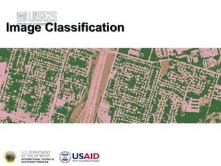
28. 28
Example: Image to be Classified

29. 29
Example: Image to be Classified
 Multiple clusters
likely represent a
single type of
“feature” on the
ground.
 Someone needs to
assign a landcover
class to all of these
clusters; can be
difficult and time
consuming.

30. 30
General Approaches to Image Classification
1. Unsupervised
2. Supervised

31. 31
Supervised Classification
Supervised classification uses image pixels representing
regions of known, homogenous surface composition --
training areas -- to classify unknown pixels.

32. 32
Supervised Classification
The underlying assumption is that spectral response of a
particular feature (i.e., land-cover class) will be relatively
consistent throughout the image.

33. 33
Advantages
Generates informational classes representing features on the
ground
 Training areas are reusable (assuming they do not change;
e.g. roads)

34. 34
Disadvantages
 Information classes may not match spectral classes
(e.g., a supervised classification of “forest” may mask the unique spectral
properties of pine and oak stands that comprise that forest)
 Homogeneity of information classes varies
 Difficulty and cost of selecting training sites
 Training areas may not encompass unique spectral classes

35. 35
Process of Supervised Classification
1. Determine a classification scheme
2. Create training areas
3. Generate training area signatures
4. Evaluate and refine signatures
5. Assign pixels to classes using a classifier (a.k.a., “decision
rule”)

36. 36
1 | Determine Classification Scheme
• Depends upon the purpose of the classification
• Make the scheme as specific as resources and available
reference data allow
You can always generalize your classification scheme to make
it less specific; making it more specific involves starting over

37. 37
2 | Create Training Areas
 Digitizing: drawing polygons around areas in the image
 Seeding: “grows” areas based on spectral similarity to seed
pixel
 Using existing data: existing maps, field data (GPS, etc.),
high-resolution imagery
 Feature space image training areas

38. 38
Training Area methods
Method Advantages Disadvantages
Digitizing
High degree of control;
can incorporate
additional imagery
May overestimate class
variance; relatively time
consuming
Seeding Auto-assisted; fast
May underestimate
class variance
Existing data
Precise map
coordinates; represents
known ground
information
May overestimate class
variance; data can be
difficult & costly to
collect

39. Selecting
ROIs
Alfalfa
Cotton
Grass
Fallow
Digitizing

40. 40
Seeding

41. 41
Training Areas “Best Practices”
 Number of pixels > 100 per class
 Individual training sites should be between 10 to 40 pixels
 Sites should be dispersed throughout the image
 Uniform and homogeneous sites

42. 42
3 | Generate Training Areas Signatures
• Signatures represent the collective spectral properties of all
the training areas defined for a particular class
• the most important step in supervised classification

43. 43
Types of Signatures
1. Parametric: signature that is based on statistical
parameters (e.g., mean) of the pixels that are in the training
area (normal distribution assumption)
2. Non-parametric: signature that is not based on statistics,
but on discrete objects (polygons or rectangles) in a feature
space image

44. 44
Parametric Signatures
e.g., mean of the
pixels that are in the
training area

45. 45
Parametric Signatures
e.g., mean of the
pixels that are in
the training area

46. 46
Non-Parametric Signatures
e.g., polygons in a
feature space

47. 47
4 | Evaluate and Refine Signatures
• Attempt to reduce or eliminate overlapping, non-
homogeneous, non-representative signatures
• Signatures should be as “spectrally distinct” as possible

48. 48
Some Signature Evaluation Methods
 Ellipse evaluation (feature space)
 Contingency matrices
 Training area histograms
 Signature plots

49. 49
Ellipse Evaluation

50. 50
Contingency analysis produces a matrix showing the
percentage of pixels that are classified correctly in a
preliminary image classification of only the training areas
 It assumes that most of the training area pixels should be
assigned to their respective land-cover class
 If a significant percentage of training pixels are classified as
another land-cover, it indicates that the spectral signatures are not
distinct enough to produce an accurate classification of the entire
image
Contingency Matrix

51. 51
Contingency Matrix
Actual Land-
cover
Classified
Land-cover Pine
Mixed
Pine
Mixed
Oak
Mixed
Fir Grass Scrub Agricult UnVeg
Pine 101 96 1 2 0 0 0 0
Mixed Pine 24 213 3 2 0 0 0 0
Mixed Oak 4 23 19 0 0 0 0 0
Mixed Fir 7 25 0 64 0 0 0 0
Grass 0 0 0 0 90 1 9 55
Scrub 0 0 0 0 2 31 0 0
Agricult. 0 0 0 0 2 0 213 57
UnVeg 0 0 0 0 5 0 14 997
Column
Total
136 357 23 68 99 32 236 1109
% Correct 74.3% 59.7% 82.6% 94.1% 90.9% 96.9% 90.3% 89.9%

52. 52
Training Area Histograms

53. 53
Signature Plots

54. 54
Signature Refinement Methods
 Refine training area boundaries
 Add/delete training areas
 Modify classification scheme/merge signatures

55. 55
Merge Signatures

56. 56
Merge Signatures

57. 57
5 | Assign Pixels to Classes
• Each pixel is independently compared to each signature
relative to the selected classification criteria, or “decision
rule”
• Pixels that satisfy the criteria for a class signature are
assigned to that class

58. 58
Classification “Decision Rules”
 Parametric: image is classified based on a statistical representation
of the data derived from the training area signatures; all image pixels
are classified
Parametric classifiers are “comprehensive”; they assign every pixel
in an image to a class (regardless of how well that pixel fits into the
classification scheme)
 Non-parametric: pixels are classified as objects in feature space;
only those pixels within the feature space object are classified

59. 59
Non-Parametric “Decision Rules”
 Parallelepiped
 Feature space

60. 60
Parallelepiped Classifier
The pixels values are compared to upper and lower limits of
each signature class (i.e., the min/max pixel values in each
band, or the mean of each band +/- 2 standard deviations)

61. 61
Parallelepiped Classifier
leave them
unclassified
or classify
them using a
parametric
classifier
• If the pixel value lies above the low
threshold and below the high threshold
for all n bands evaluated, it is assigned
to that class
• When an unknown pixel does not
satisfy any of the criteria, it is assigned
to an unclassified category
• We can visually see the two-
dimensional box, but this could be
extended to n dimensions.

62. 62
• Landsat TM training statistics for five
classes measured in bands 4 and 5
displayed as cospectral parallelepipeds.
• The upper and lower limit of each
parallelepiped is ±1s, superimposed on a
feature space plot of bands 4 and 5.
• Band 4: confusion between class 1 and 4
• Band 5: confusion between class 3 and 4
• Both band 4 and 5: separate all 5 classes
at ±1s
Parallelepiped Classifier

63. 63
Parallelepiped Classifier
 Advantages: fast; good for non-normal distributions; can
limit classification to specific land cover
 Disadvantages: classes can include pixels spectrally distant
from the signature mean; does not incorporate variability;
not all pixels are classified; allows class overlap

64. 64
Feature Space Classifier
Classifies pixels that fall within non-parametric signatures
identified in the feature space image not used very often
because it is difficult to accurately create and evaluate non-
parametric signatures

65. 65
Feature Space Classifier
non-
parametric
signatures
you decide
how they
are handled

66. 66
Feature Space Classifier
 Advantages: good for non-normal distributions and multi-
modal signatures (that include many land cover features)
 Disadvantages: feature space images are difficult to
interpret; allows class overlap

67. 67
Parametric “Decision Rules”
 Minimum distance
 Maximum likelihood

68. 68
Minimum Distance Classifier
Classifies pixels based on the spectral distance between the
candidate pixel and the mean value of each signature (class)
in each image band

69. 69
Minimum Distance Classifier
mean value of
each class

70. Minimum Distance Classifier
• The vectors (arrows)
represent the distance
from candidate pixels a
and b to the mean of
all classes in a
minimum distance to
means classification
algorithm
• Pixel a – Forest
• Pixel b - Wetland

71. 71
Minimum Distance Classifier
 Advantages: fast; no unclassified pixels
 Disadvantages: does not incorporate variability of
signatures
 In most cases, a maximum likelihood classifier is a better
choice

72. 72
Maximum Likelihood Classifier
• Classifies pixels based on the probability that a pixel falls
within a certain class
• If you know that the probabilities are not equal for all
classes, you can specify weight factors
 For example, if you know that a large percentage of a particular
image area is forested, you may want to weight that class with a
higher probability than other classes

73. Maximum Likelihood Classifier
• Probability of an
unknown pixel being
one of the classes
• If an unknown pixel has
brightness values within
the wetland region, it
has a high probability of
being wetland

74. Maximum Likelihood Classifier
pixel X would be
assigned to forest
because the probability
is greater for forest
than for agriculture.
The ellipses represent
standard deviations
from the mean
Minimum distance
classifier - Agriculture

75. 75
Maximum Likelihood Classifier
 Advantages: most accurate; considers variability
 Disadvantages: slow; relies heavily on normally distributed
signatures

76. Example: Image to be Classified

77. Training Data Selection

78. Supervised Classification Results

79. Supervised classification. Identify known a
priori through a combination of fieldwork,
map analysis, and personal experience as
training sites; the spectral characteristics of
these sites are used to train the
classification algorithm for eventual land-
cover mapping of the remainder of the
image. Every pixel both within and outside
the training sites is then evaluated and
assigned to the class of which it has the
highest likelihood of being a member.
Unsupervised classification, The
computer or algorithm automatically
group pixels with similar spectral
characteristics (means, standard
deviations, covariance matrices,
correlation matrices, etc.) into unique
clusters according to some statistically
determined criteria. The analyst then
re-labels and combines the spectral
clusters into information classes.

80. 80
Final Thoughts on Supervised Classification
 Accuracy vs. Precision
 Land cover vs. land use

81. 81
Accuracy & Precision

82. 82
Accuracy & Precision

83. 83
Accuracy & Precision

84. Accuracy & Precision
Relationship between the level of
detail required and the spatial
resolution of representative
remote sensing systems for
vegetation inventories.

85. 85
Land Cover vs. Land Use
• Land cover refers to the type of material present on the landscape (e.g.,
water, sand, crops, forest, wetland, human-made materials such as
asphalt).
• Land use refers to what people do on the land surface (e.g., agriculture,
commerce, settlement).

86. 86
The U.S. Geological Survey’s
Land-Use/Land-Cover Classification
System for Use with Remote Sensor
Data
Land Cover vs. Land Use

87. 87
Hard vs. Fuzzy Classification
 Supervised and unsupervised classification algorithms
typically use hard classification logic to produce a
classification map that consists of hard, discrete categories
(e.g., forest, agriculture).
 Fuzzy classification logic, takes into account the
heterogeneous and imprecise nature (mix pixels) of the real
world.
Proportion of the m classes within a pixel (e.g., 10% bare soil,
10% shrub, 80% forest). Fuzzy classification schemes are not
currently standardized.

89. 89
Pixel-based vs. Object-oriented Classification
 Processing the entire scene pixel by pixel. This is commonly
referred to as per-pixel (pixel-based) classification.
 Object-oriented classification techniques allow the analyst to
decompose the scene into many relatively homogenous image
objects (referred to as patches or segments) using a multi-
resolution image segmentation process
 Object-oriented classification based on image segmentation is
often used for the analysis of high-spatial-resolution imagery
(e.g., 1  1 m Space Imaging IKONOS and 0.61  0.61 m Digital
Globe QuickBird)