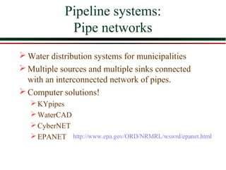
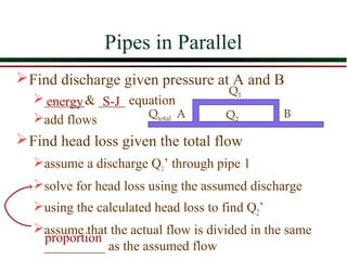
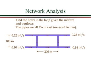
The document discusses pipe networks for water distribution systems. It describes: 1) Pipe networks can have multiple sources and sinks connected by an interconnected network of pipes. Computer solutions are used to model pipe networks. 2) Assumptions made in modeling pipe networks include each point having a single pressure and equal pressure changes along parallel paths. Conservation of mass is assumed at nodes. 3) Pipes can be modeled in parallel by applying the energy equation between nodes and adding pipe flows. Computer solutions are needed for networks with multiple loops.

1. 
Pipe Networks
Pipeline systems
Transmission lines
You are here Pipe networks
Measurements
Manifolds and diffusers
Pumps
Transients
School of Civil and
Monroe L. Weber-Shirk Environmental Engineering

2. Pipeline systems:
Pipe networks
 Water distribution systems for municipalities
 Multiple sources and multiple sinks connected
with an interconnected network of pipes.
 Computer solutions!
 KYpipes
 WaterCAD
 CyberNET
 EPANET http://www.epa.gov/ORD/NRMRL/wswrd/epanet.html

3. Water Distribution System
Assumption
 Each point in the a
system can only
have one pressure
_______ 1 2
 The pressure change
from 1 to 2 by path a
must equal the b
pressure change
from 1 to 2 by path b
p1 V12 p2 V22
+ + z1 = + + z 2 + hL
γ 2g γ 2g
2
p 2 p1 V1 V22
− = + z1 −
a a
− z2 − hL Same for path b!
γ γ 2g 2g a

4. Water Distribution System
Assumption
V12 V22 V12 V22
a
+ z1 − a
− z2 − hL = b
+ z1 − b
− z 2 − hL
2g 2g a
2g 2g b
a
1 2
Pressure change by path a
b
hL = hL
a b
zero
Or sum of head loss around loop is _____.
(Need a sign convention)
 Pipe diameters are constant or K.E. is small
 Model withdrawals as occurring at nodes so
V is constant between nodes

5. Pipes in Parallel
 Find discharge given pressure at A and B
Q1
______& ____ equation
energy S-J
add flows Qtotal A Q2 B
 Find head loss given the total flow
assume a discharge Q1’ through pipe 1
solve for head loss using the assumed discharge
using the calculated head loss to find Q2’
assume that the actual flow is divided in the same
proportion
_________ as the assumed flow

6. Networks of Pipes
Mass __________ at all nodes
____ conservation 0.32 m /s
3
A
0.28 m3/s
 The relationship between head ?
loss and discharge must be
maintained for each pipe
Darcy-Weisbach equation
Swamee-Jain
_____________
Exponential friction formula a
_____________
Hazen-Williams 1 2
b

7. Network Analysis
Find the flows in the loop given the inflows
and outflows.
The pipes are all 25 cm cast iron (ε=0.26 mm).
0.32 m3/s A B 0.28 m3/s
100 m
0.10 m3/s C D
0.14 m3/s
200 m

8. Network Analysis
 Assign a flow to each pipe link
 Flow into each junction must equal flow out
of the junction
arbitrary
0.32 m3/s A B 0.28 m3/s
0.32
0.00 0.04
0.10 m3/s C D
0.14 m3/s
0.10

9. Network Analysis
h f = 34.7m
 Calculate the head loss in each pipe 1
h f = 0.222m
 8 fL  2 2
hf =  
5 2 Q f=0.02 for Re>200000 h f = −3.39m
 gD π  3
h f = kQ Q Sign convention +CW h f = −0.00m
4
4
 8(0.02)(200)  s 2 k1,k3=339
k1 =   = 339
 (9.8)(0.25) 5 π 2  m5 k2,k4=169
∑h fi = 31.53m
  i=1
0.32 m3/s A 1 B 0.28 m3/s
4 2
0.10 m3/s C 3 D
0.14 m3/s

10. Network Analysis
 The head loss around the loop isn’t zero
 Need to change the flow around the loop
clockwise
 the ___________ flow is too great (head loss is
positive)
 reduce the clockwise flow to reduce the head loss
 Solution techniques
optimizes correction
 Hardy Cross loop-balancing (___________ _________)
 Use a numeric solver (Solver in Excel) to find a change
in flow that will give zero head loss around the loop
 Use Network Analysis software (EPANET)

11. Numeric Solver
 Set up a spreadsheet as shown below.
 the numbers in bold were entered, the other cells are
calculations
 initially ∆Q is 0
 use “solver” to set the sum of the head loss to 0 by changing ∆Q
 the column Q0+ ∆Q contains the correct flows
∆Q 0.000
pipe f L D k Q0 Q0+∆Q hf
P1 0.02 200 0.25 339 0.32 0.320 34.69
P2 0.02 100 0.25 169 0.04 0.040 0.27
P3 0.02 200 0.25 339 -0.1 -0.100 -3.39
P4 0.02 100 0.25 169 0 0.000 0.00
Sum Head Loss 31.575

12. Solution to Loop Problem
Q0+ ∆Q
0.218
−0.062
−0.202
−0.102
0.32 m3/s A 1 B 0.28 m3/s
4 0.218 2
0.102 0.062
0.202
0.10 m /s3 C 3 D
0.14 m3/s
Better solution is software with a GUI showing the pipe network.

13. Network Elements
 Controls
 Check valve (CV)
 Pressure relief valve
 Pressure reducing valve (PRV)
 Pressure sustaining valve (PSV)
 Flow control valve (FCV)
 Pumps: need a relationship between flow and head
 Reservoirs: infinite source, elevation is not
affected by demand
 Tanks: specific geometry, mass conservation
applies

14. Check Valve
 Valve only allows flow in one direction
 The valve automatically closes when flow
begins to reverse
open closed

15. Pressure Relief Valve
closed open
pipeline
relief flow
Low pipeline pressure High pipeline pressure
Valve will begin to open when pressure in
exceeds
the pipeline ________ a set pressure
(determined by force on the spring).
Where high pressure could cause an explosion (boilers, water heaters, …)

16. Pressure Regulating Valve
sets maximum pressure downstream
closed open
High downstream pressure Low downstream pressure
Valve will begin to open when the pressure
___________ less
downstream is _________ than the setpoint
pressure (determined by the force of the spring).
Similar function to pressure break tank

17. Pressure Sustaining Valve
sets minimum pressure upstream
closed open
Low upstream pressure High upstream pressure
Valve will begin to open when the pressure
upstream greater
________ is _________ than the setpoint pressure
(determined by the force of the spring).
Similar to pressure relief valve

18. Flow control valve (FCV)
 Limits the flow rate
____ ___
through the valve to a
specified value, in a
specified direction
 Commonly used to limit
the maximum flow to a
value that will not
adversely affect the
provider’s system

19. Pressure Break Tanks
 In the developing world small water supplies in
mountainous regions can develop too much
pressure for the PVC pipe.
 They don’t want to use PRVs because they are too
expensive and are prone to failure.
 Pressure break tanks have an inlet, an outlet, and
an overflow.
 Is there a better solution?

20. Network Analysis Extended
 The previous approach works for a simple
loop, but it doesn’t easily extend to a whole
network of loops
 Need a matrix method
Initial guess for flows
Adjust all flows to reduce the error in pressures
 __________________________
Simultaneous equations
 _______________________________
Appendix D of EPANET manual

21. Pressure Network Analysis
Software: EPANET
reservoir
pipe junction
0.32 m3/s A 1 B 0.28 m3/s
4 0.218 2
0.102 0.062
0.202
0.10 m /s
3 C 3 D
0.14 m3/s

22. EPANET network solution
 8 fL  2 H i − H j = hij = rQij + mQij
n 2
hf =  
5 2 Q
 gD π 
∑Qj
ij − Di = 0
 8 fL 
r =
 gD 5π 2 ÷

AH = F
Aii = ∑ pij
n=2 j
Aij = − pij
1
pij = 1
 8 fL  pij = n −1
2 Q
5 2 ÷ ij nr Qij + 2m Qij
 gD π 

23.  
Fi =  ∑ Qij − Di ÷+ ∑ yij + ∑ pif H f
 j  j f
( n
yij = pij r Qij + m Qij
2
) sgn ( Q )
ij
Qij = Qij −  yij − pij ( H i − H j ) 
 