Downloaded 501 times


![Hardy Cross Method:-
• To analyze a given distribution system to determine the pressure and flow available in any section of the
system and to suggest improvement if needed a number of methods are used like Equivalent pipe, Circle
method, method of section and Hardy-cross method. Hardy-cross method is a popular method. According
to this method the sum of the loss of head for a closed network / loop is equal to zero. Also the sum of
inflow at a node / joint is equal to the out flow i.e. Σinflow = Σoutflow or total head loss = 0
Assumption:-
Sum of the inflow at a node/point is equal to outflow. Σinflow = Σoutflow; Σtotal flow = 0
Algebraic sum of the head losses in a closed loop is equal to zero. Σhead losses = 0
Clockwise flows are positive. Counter clockwise flows are negative.
• Derivation:-
According to Hazen William Equation H= 10.68 (Q/C) 1.85 (L / d)4.87
H= KQ1.85 where K = (10.68L)/(C1.85*d4.87)
For any pipe in a closed loop
Q = Q+ Δ where Q = actual flow; Q= assumed flow and Δ = required flow correction
1 1 H= KQx (i) x is an exponent whose value is generally 1.85
From (i) H = K(Q+ Δ)x By Binomial theorm = K[Qx + (xQx-1Δ)/1! + {x(x-1)Qx-2Δ2}/2! + ……..]
1 1
1
As Δ is very small as compared to Q, we can neglect Δ2 etc. Therefore, H = KQ1
x + KxQ1
x-1Δ (ii)
For a closed loop Σ H = 0 => Σ Qx = 0 => Σ k Q1
x = - ΔΣ x Q1
x-1) => Δ = - Σ k Q1
x / (Σ x Q1
x-1)](https://image.slidesharecdn.com/hardycrossmethod-141103083149-conversion-gate01/85/Hardycross-method-2-320.jpg)
![As H = K*Q x
Σ KQ1
x/ Q1 = H/Q 1
Therefore, Δ = - Σ H/ [x* Σ (H)/ Q1]
Above equation is used in Hardy Cross Method
Procedure : (i) Assume the diameter of each pipe in the loop.
(ii) Assume the flow in the pipe such that sum of the inflow = sum of the outflow at any junction or node
( V = V1 + V2 or Q = Q1 + Q2 )
(iii) Compute the head losses in each pipe by Hazen William Equation H = 10.68 * (Q/C)1.85 * L/D4.87
(iv) Taking clock wise flow as positive and anti clock wise as negative.
(v) Find sum of the ratio of head loss and discharge in each pipe without regard of sign Σ ( H/Q1 )
(vi) Find the correction for each loop from Δ = - Σ H/ [x* Σ (H)/ Q1] and apply it to all pipes.
(vii) Repeat the procedure with corrected values of flow and continue till the correction become very small](https://image.slidesharecdn.com/hardycrossmethod-141103083149-conversion-gate01/85/Hardycross-method-3-320.jpg)
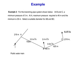
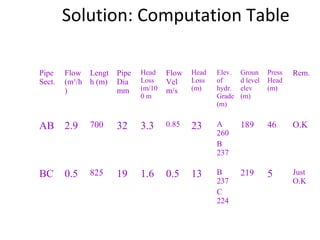
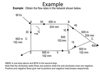
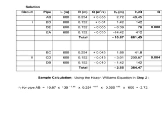

The document discusses the Hardy Cross Method for analyzing water distribution systems to determine pressures and flows. It involves the following steps: 1. Assume pipe diameters and initial flows such that the sum of inflows equals outflows at junctions. 2. Calculate head losses in each pipe using the Hazen-Williams equation. 3. Calculate flow corrections using an equation that sets the sum of head losses around loops to zero. 4. Repeat using corrected flows until flow corrections become small. An example problem applies the method to determine suitable pipe diameters for a branching system given pressure requirements at nodes.