Open channel Flow

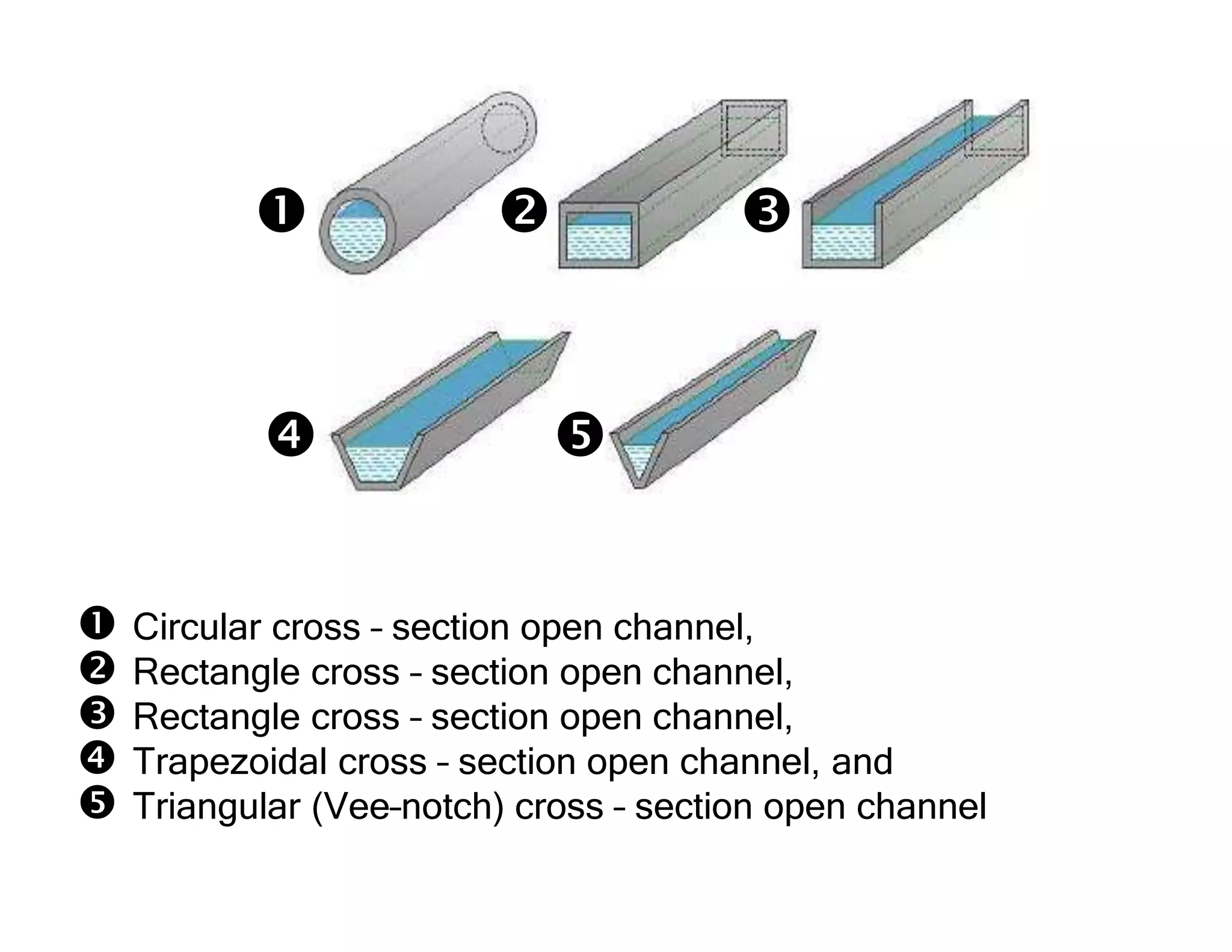
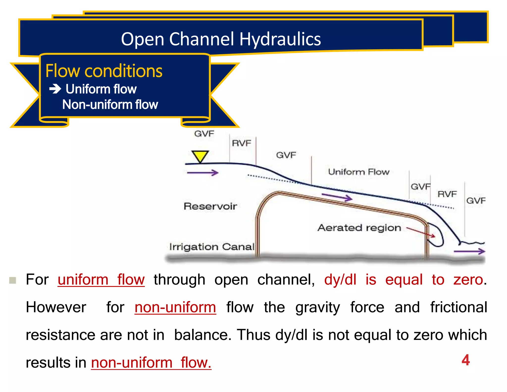
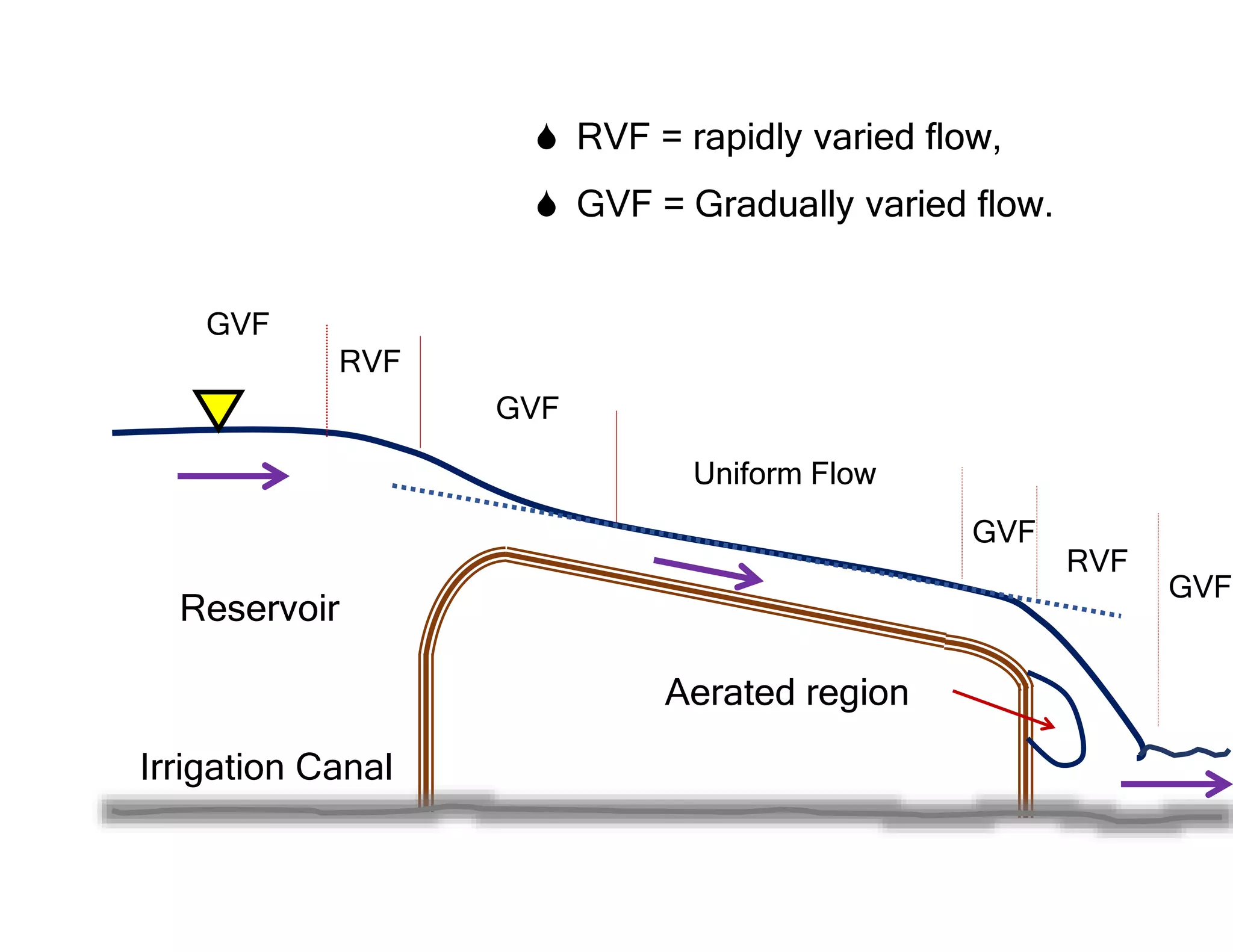
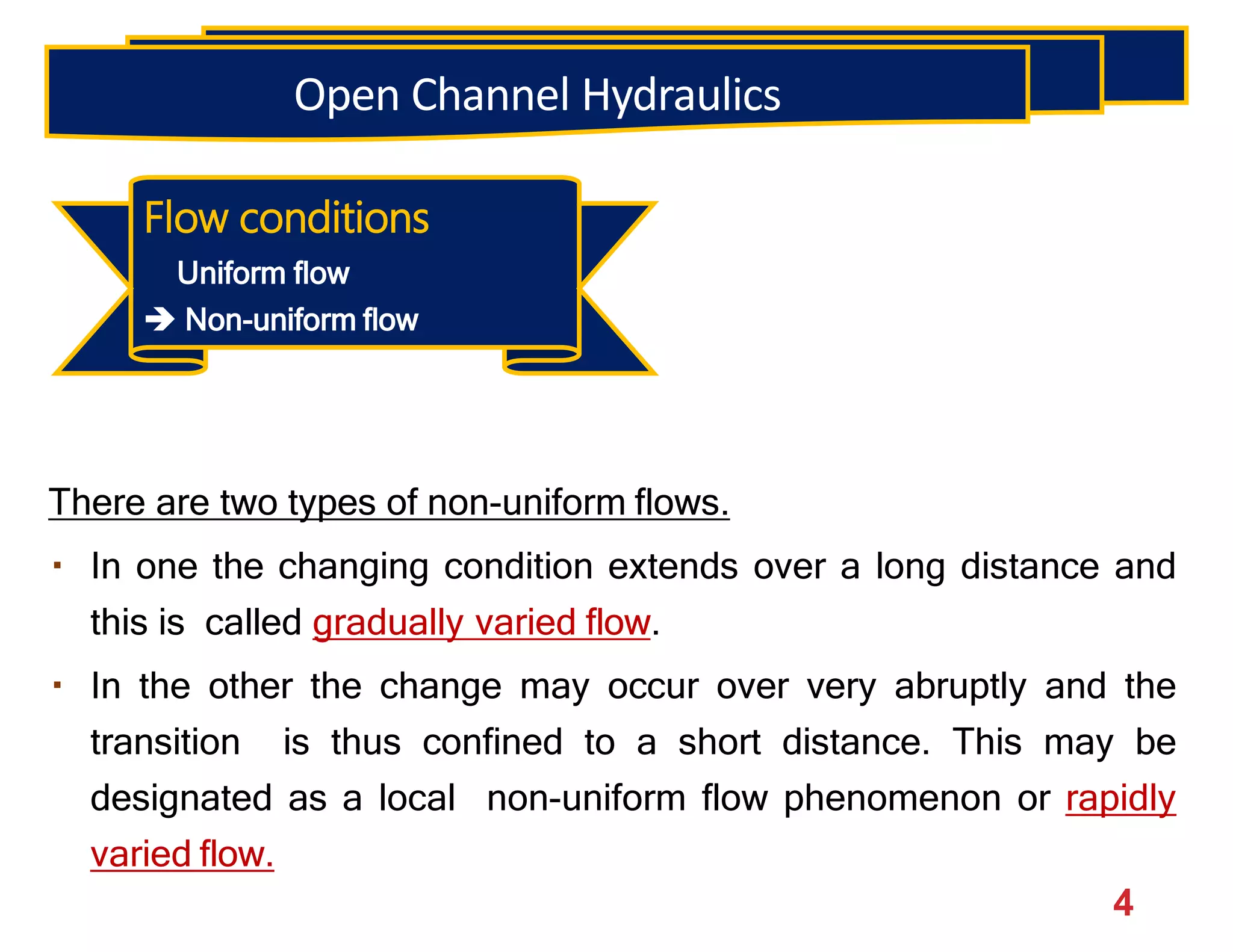
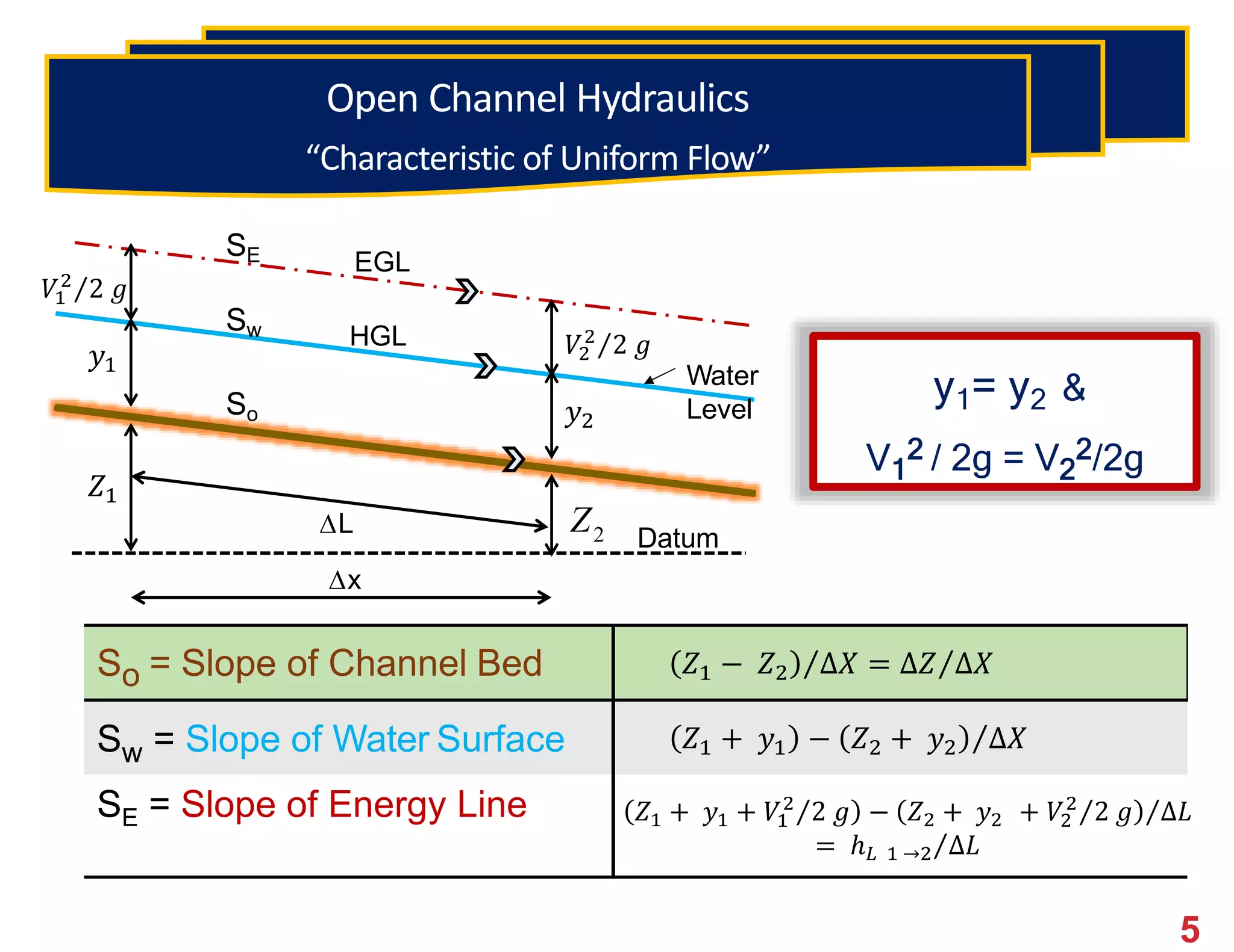
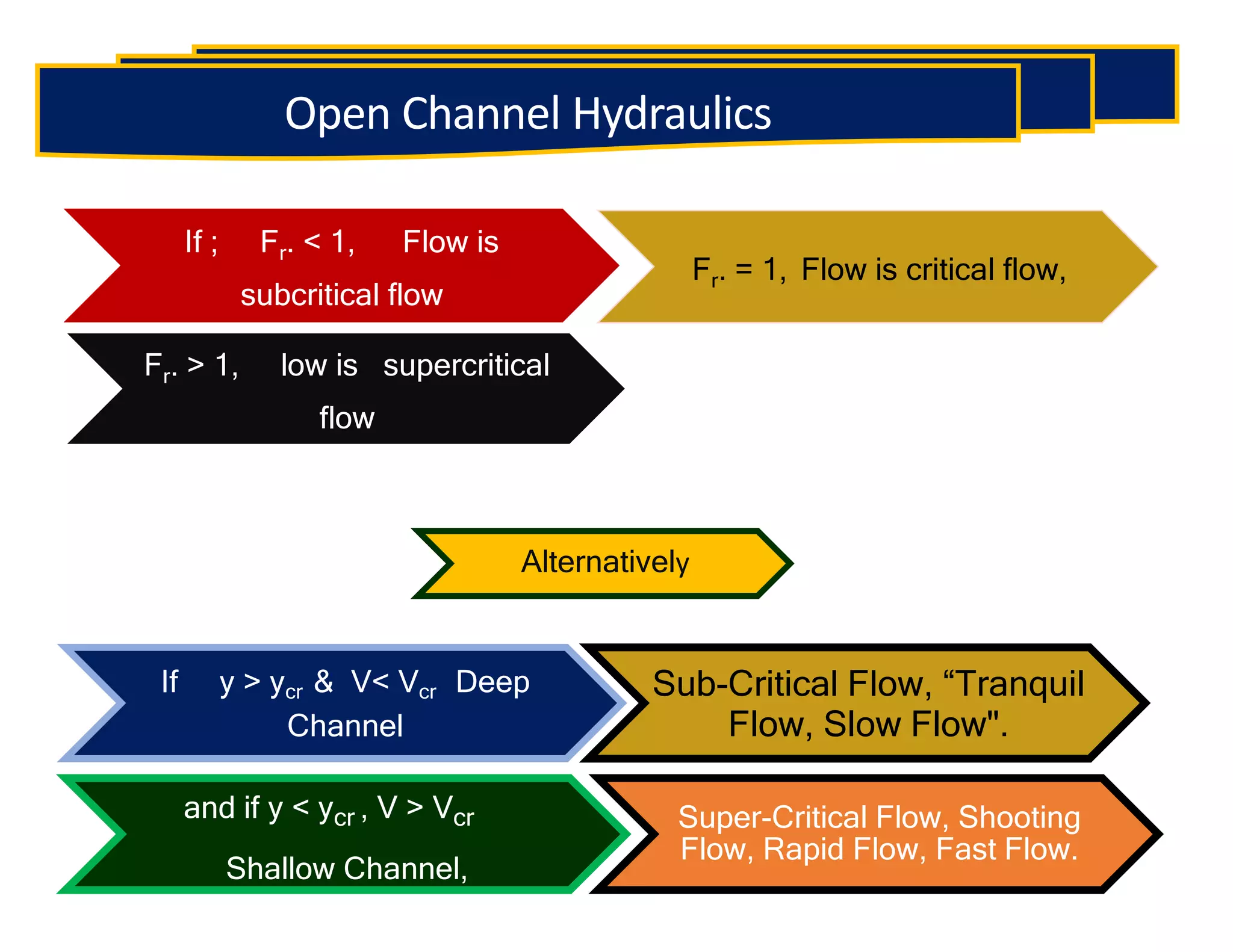
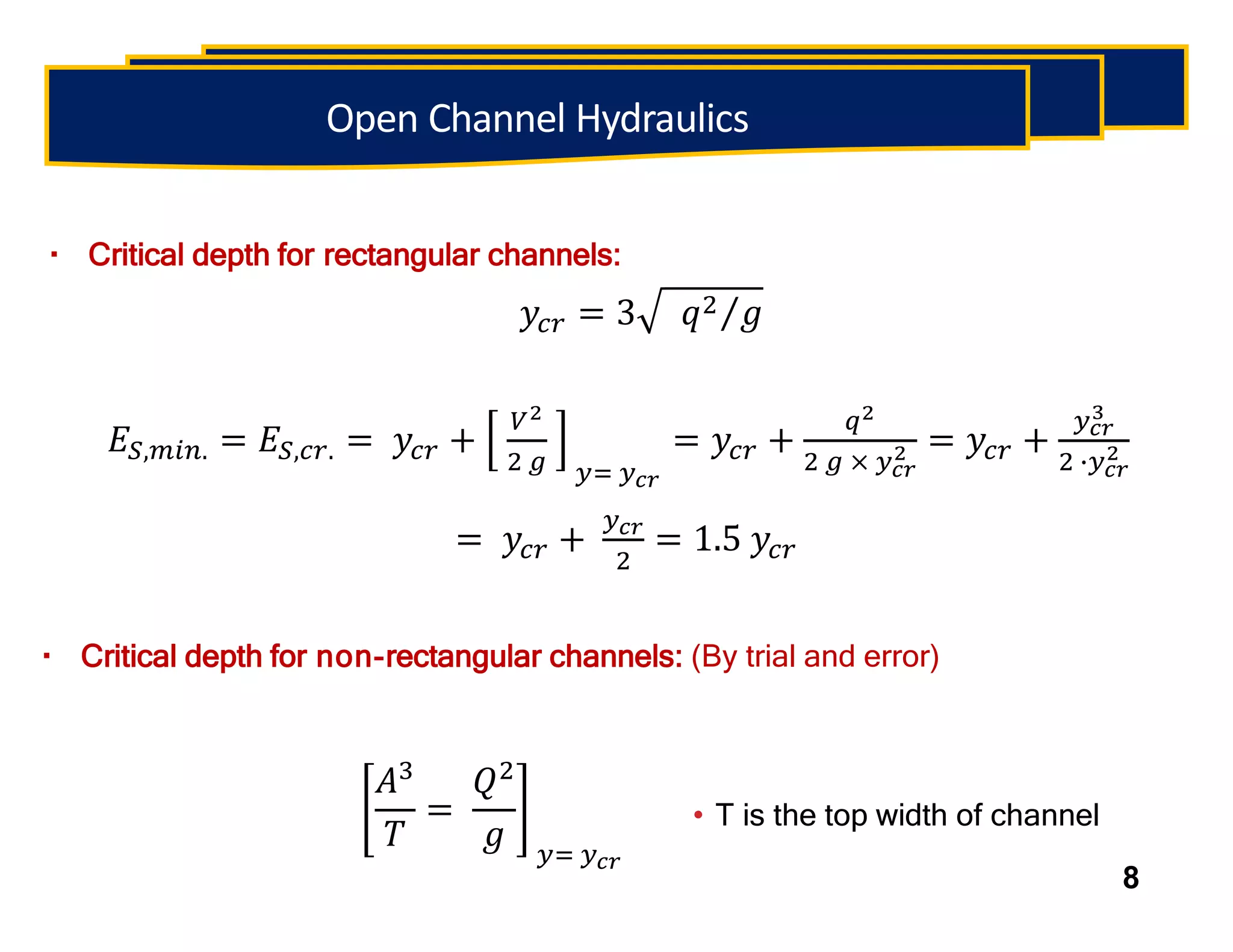
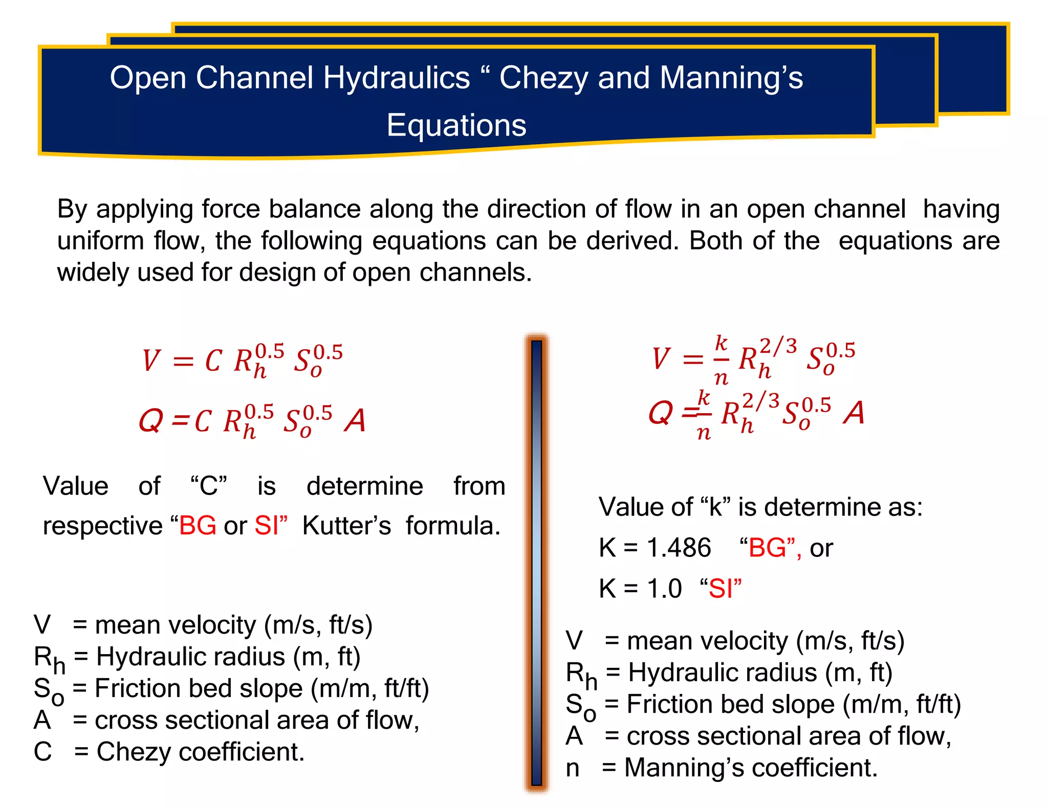
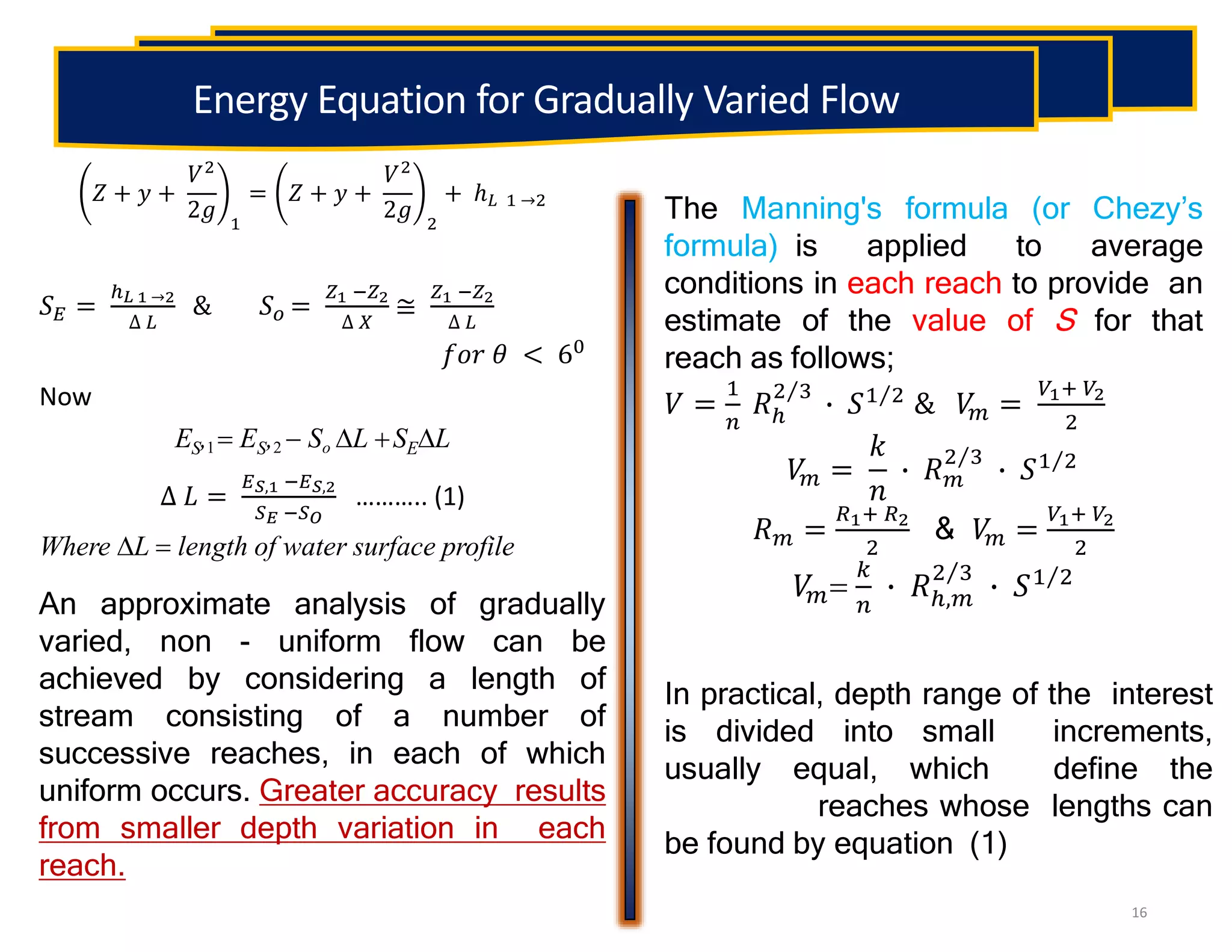
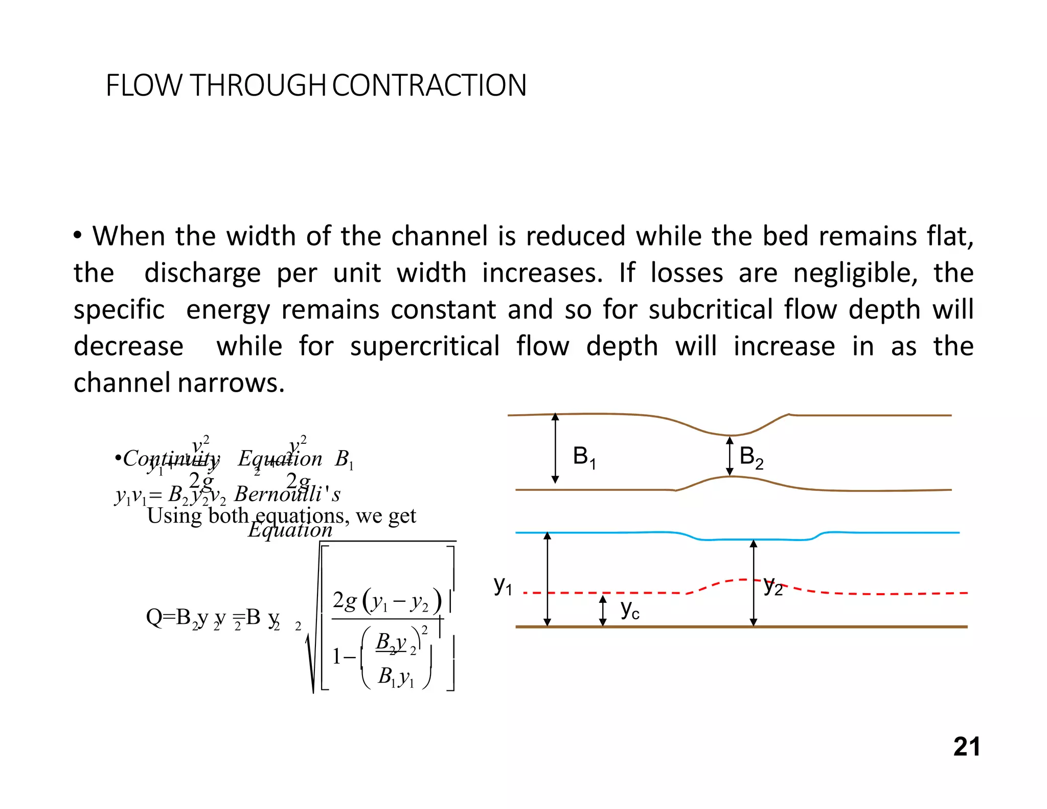
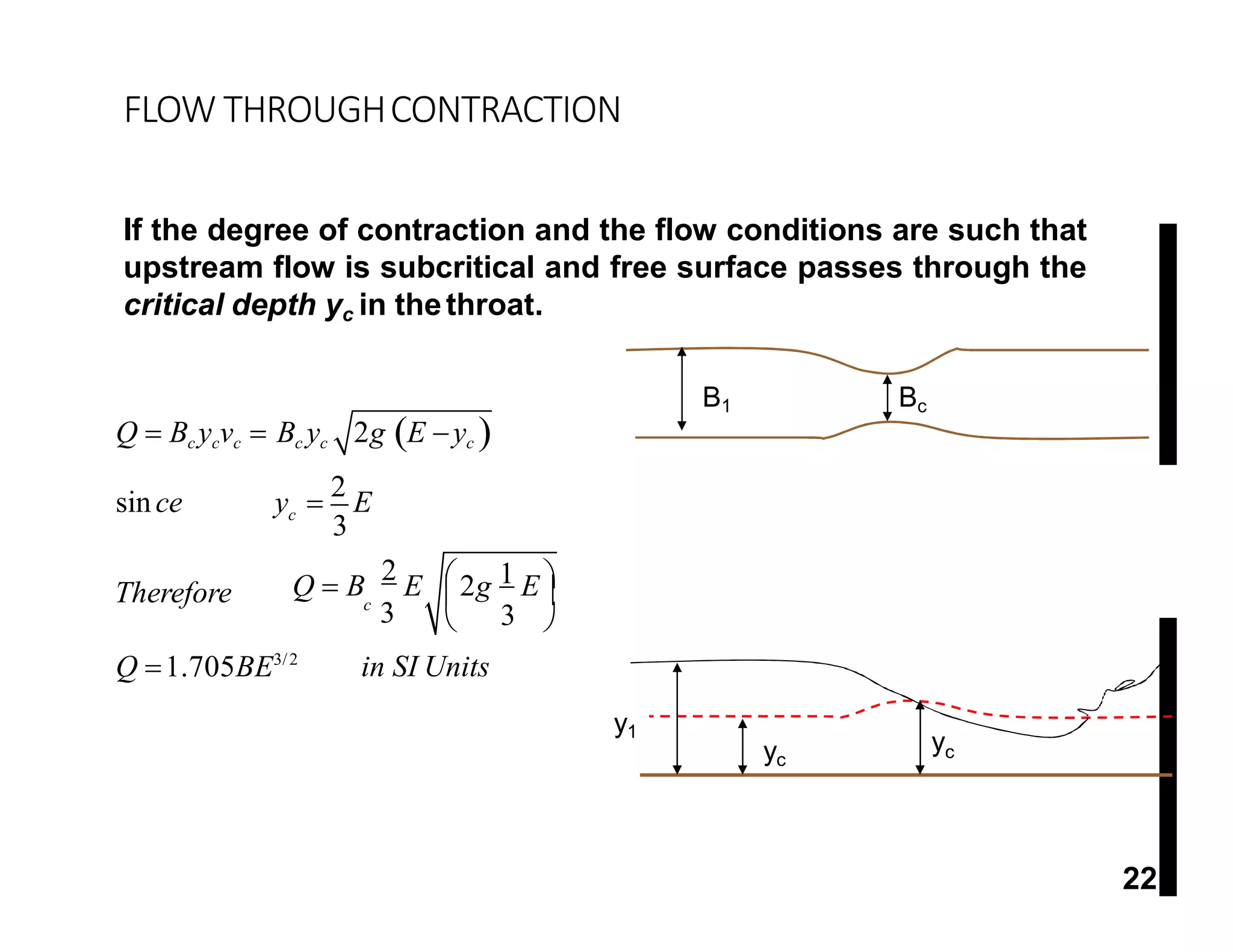
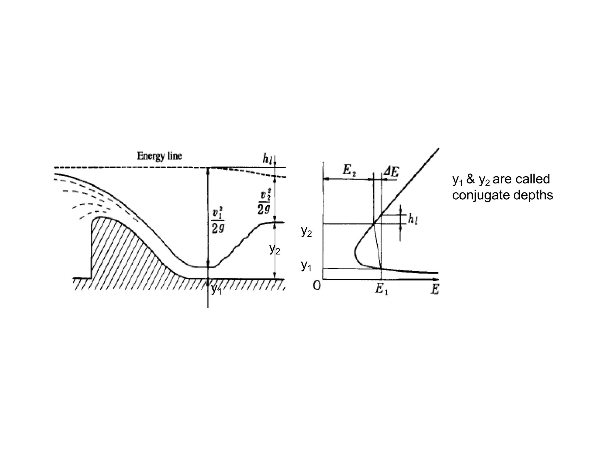
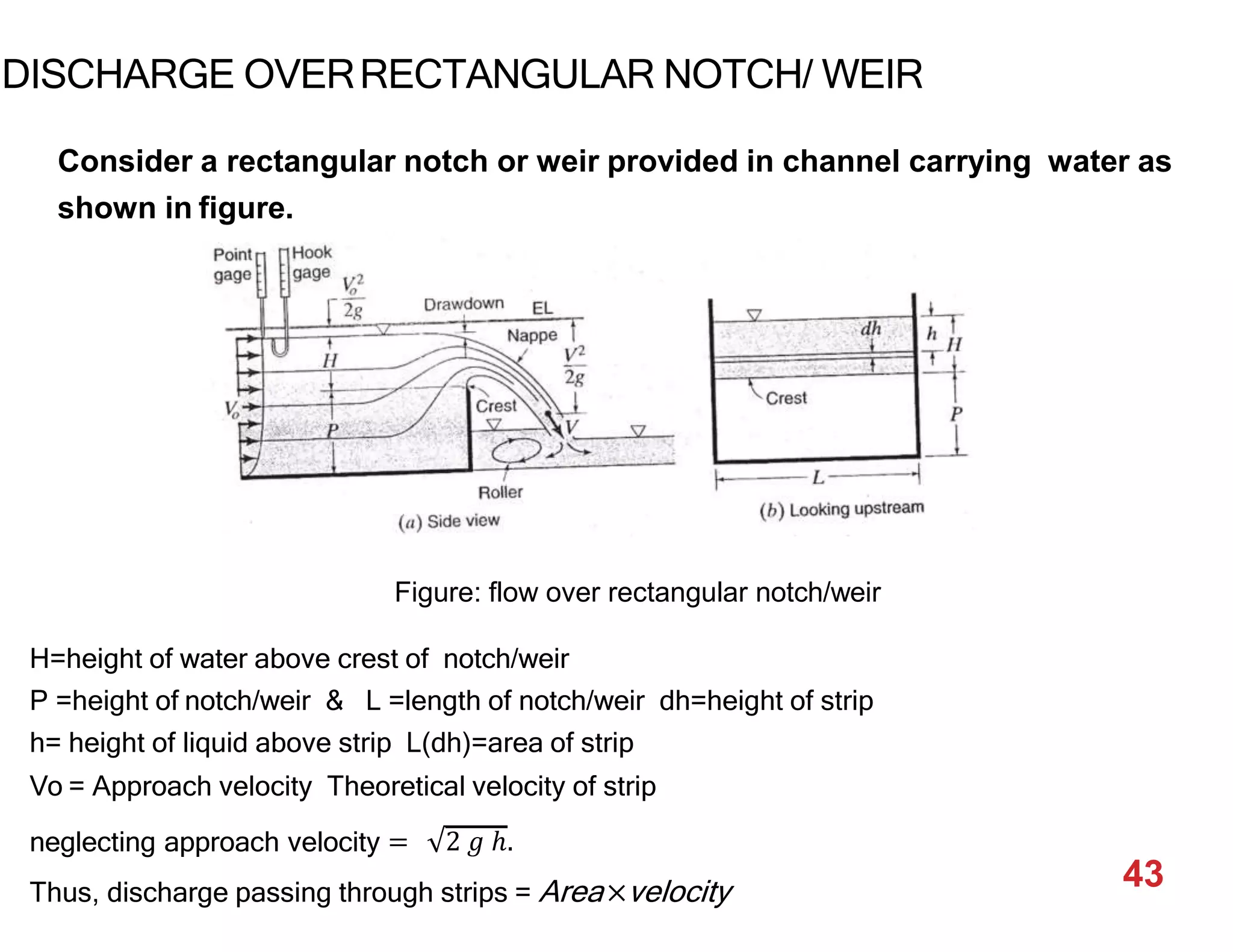
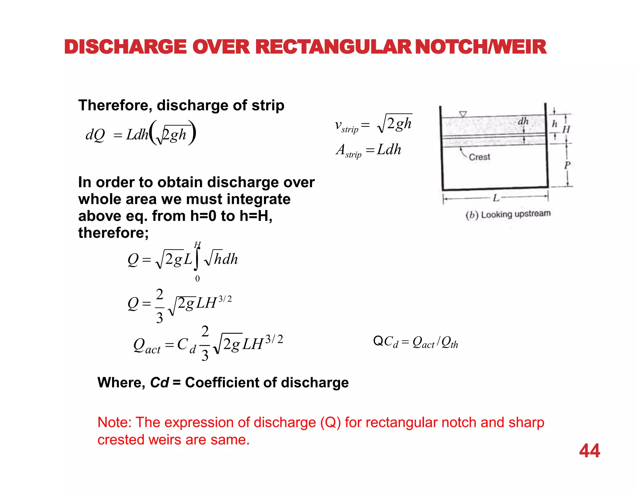
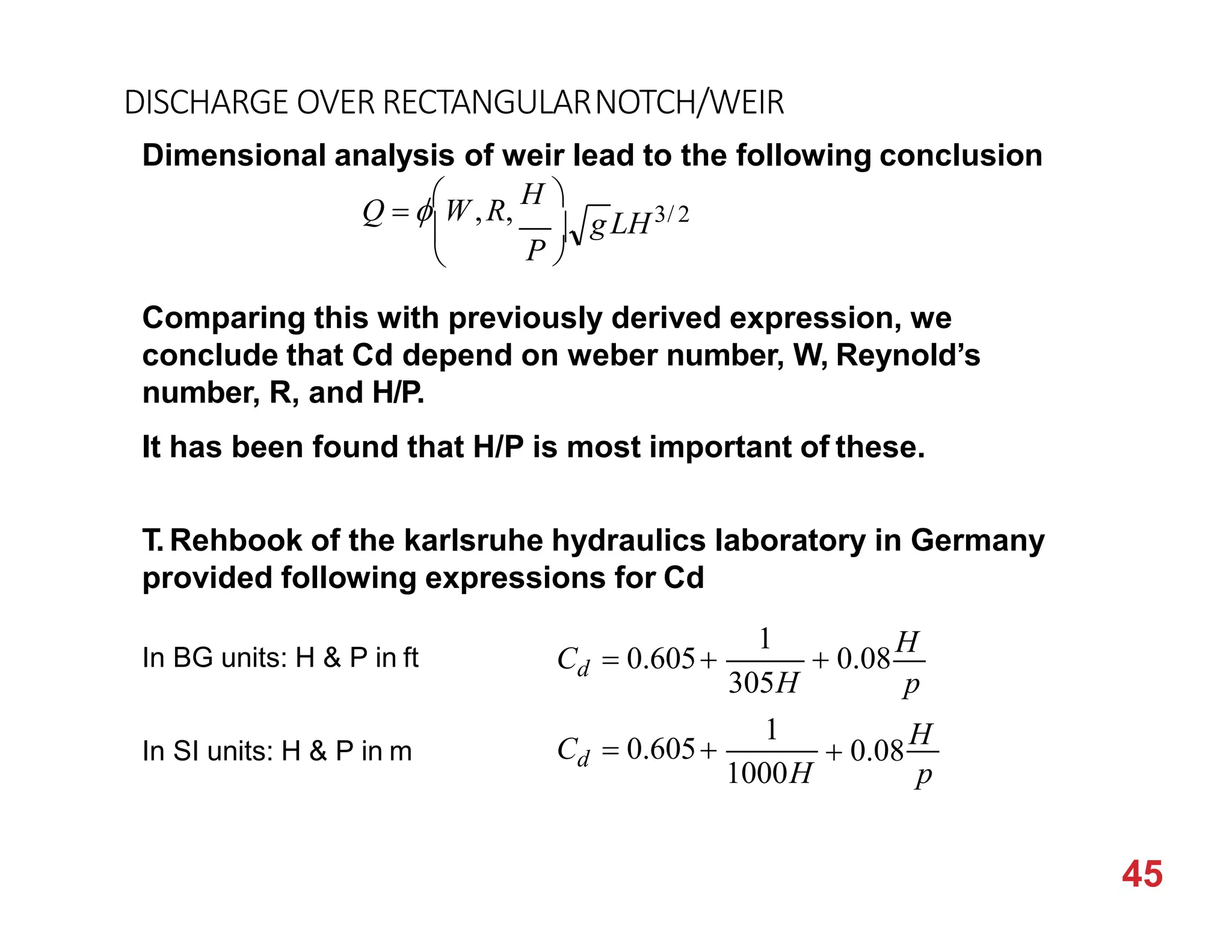
1
REVIEWOFOPENCHANNEL HYDRAULICS and
THEORY OF DISCHARGE MEASURING
STRUCTURES

2
After completing this lecture…The students should be
able to:
 Understand the behavior of open channel flow under various
conditions
 Learn the basic theories that govern the design of open
channels and hydraulic structures
 Apply the basic theories to derive various formula used in the
design calculation of hydraulic structures such as weir/notches
 References:
Fluid Mechanics With Engineering Applications, 10TH ED, By E.
Finnemore and Joseph Franzini, McGraw Hills
Learning Output

 An open channel is the one in which stream is not complete
enclosed by solid boundaries and therefore has a free surface
subjected only to atmosphere pressure.
 The flow in such channels is not caused by some external head,
but rather only by gravitational component along the slope of
channel. Thus open channel flow is also referred to as free
surface flow or gravity flow.
 Examples of open channel are:
 Rivers, canals, streams, & sewerage system etc….
3
Open Channel Hydraulics

  
 
 Circular cross – section open channel,
 Rectangle cross – section open channel,
 Rectangle cross – section open channel,
 Trapezoidal cross – section open channel, and
 Triangular (Vee–notch) cross – section open channel

 For uniform flow through open channel, dy/dl is equal to zero.
However for non-uniform flow the gravity force and frictional
resistance are not in balance. Thus dy/dl is not equal to zero which
results in non-uniform flow. 4
Flow conditions
 Uniform flow
Non-uniform flow

Irrigation Canal
Reservoir
Aerated region
Uniform Flow
GVF
RVF
GVF
GVF
RVF
GVF
 RVF = rapidly varied flow,
 GVF = Gradually varied flow.

There are two types of non-uniform flows.
In one the changing condition extends over a long distance and
this is called gradually varied flow.
In the other the change may occur over very abruptly and the
transition is thus confined to a short distance. This may be
designated as a local non-uniform flow phenomenon or rapidly
varied flow.
4
Flow conditions
Uniform flow
 Non-uniform flow

Datum
So
2
Z
HGL
EGL
Water
Level
Sw
∆L
∆x
5
“Characteristic of Uniform Flow”
SE
𝑦2
𝑉2
2
2 𝑔
𝑉1
2
2 𝑔
𝑦1
𝑍1
y1= y2 &
V1
2 / 2g = V2
2/2g
So = Slope of Channel Bed
Sw = Slope of Water Surface
SE = Slope of Energy Line
𝑍1 + 𝑦1 − 𝑍2 + 𝑦2 ∆𝑋
𝑍1 + 𝑦1 + 𝑉1
2
2 𝑔 − 𝑍2 + 𝑦2 + 𝑉2
2
2 𝑔 ∆𝐿
= ℎ𝐿 1 →2 ∆𝐿
𝑍1 − 𝑍2 ∆𝑋 = ∆𝑍 ∆𝑋

For Uniform Flow : y1= y2 & V1
2/2g = V2
2/2g
Hence the line indicating the bed of the channel, water surface
profile and energy line are parallel to each other.
For θ being very small (say less than 5 degree) i.e. ∆x=∆L
So = Sw = SE

Energy Equation:
𝑍 + 𝑦 +
𝑉2
2𝑔 1
= 𝑍 + 𝑦 +
𝑉2
2𝑔 2
+ ℎ𝐿 1 →2
Let’s assume two section close to each 1other (neglecting head loss) and take
bed of channel as datum, above equation can be rewritten as
𝑦 +
𝑉2
2𝑔 1
= 𝑦 +
𝑉2
2𝑔 2
Specific Energy
At a section in an open channel is the energy with reference to the bed of the
channel 𝐸𝑆 = 𝑦 +
𝑉2
2𝑔
Mathematically;
𝐸𝑠 = 𝑦 +
𝑉2
2 𝑔
= 𝑦 +
𝑞2
2 𝑔
(For a rectangular Channel)
where ES,1 and ES,2 are called specific energy at 1 and 2.
6

As it is clear from ES~y diagram drawn for constant discharge for any given value
of E, there would be two possible depths, say y1 and y2. These two depths are
called Alternate depths.
However for point “C” corresponding to minimum specific energy 𝐸𝑠,𝑚𝑖𝑛. there
would be only one possible depth ycr. The depth ycr is know as critical depth.
The critical depth may be defined as depth corresponding to minimum specific
energy discharge remaining Constant
𝐸𝑆 = 𝑦 +
𝑞2
2 𝑔 𝑦2
𝑤ℎ𝑒𝑟𝑒 𝑞 = 𝑄 𝐵

Types of flow in open channels
Subcritical, Critical and Supercritical Flow: These are classified with Froude
number.
Froude No. (Fr): It is ratio of inertial force to gravitational force of flowing fluid.
Mathematically, Froude no. is
𝐹𝑟 =
𝑉
𝑔 𝑦ℎ
where, V is average velocity of flow, h is depth of flow and g is gravitational
acceleration

If ; Fr. < 1, Flow is
subcritical flow
Fr. = 1, Flow is critical flow,
Fr. > 1, low is supercritical
flow
Alternatively
If y > ycr & V< Vcr Deep
Channel
Sub-Critical Flow, “Tranquil
Flow, Slow Flow".
and if y < ycr , V > Vcr
Shallow Channel,
Super-Critical Flow, Shooting
Flow, Rapid Flow, Fast Flow.

Critical depth for rectangular channels:
• T is the top width of channel
8
𝑦𝑐𝑟 = 3 𝑞2 𝑔
𝐸𝑆,𝑚𝑖𝑛. = 𝐸𝑆,𝑐𝑟. = 𝑦𝑐𝑟 +
𝑉2
2 𝑔 𝑦= 𝑦𝑐𝑟
= 𝑦𝑐𝑟 +
𝑞2
2 𝑔 × 𝑦𝑐𝑟
2 = 𝑦𝑐𝑟 +
𝑦𝑐𝑟
3
2 ∙𝑦𝑐𝑟
2
= 𝑦𝑐𝑟 +
𝑦𝑐𝑟
2
= 1.5 𝑦𝑐𝑟
Critical depth for non-rectangular channels: (By trial and error)
𝐴3
𝑇
=
𝑄2
𝑔 𝑦= 𝑦𝑐𝑟

Open Channel Hydraulics “ Chezy and Manning’s
Equations
By applying force balance along the direction of flow in an open channel having
uniform flow, the following equations can be derived. Both of the equations are
widely used for design of open channels.
𝑉 = 𝐶 𝑅ℎ
0.5
𝑆𝑜
0.5
Q = 𝐶 𝑅ℎ
0.5
𝑆𝑜
0.5 A
Value of “C” is determine from
respective “BG or SI” Kutter’s formula.
V = mean velocity (m/s, ft/s)
Rh = Hydraulic radius (m, ft)
So = Friction bed slope (m/m, ft/ft)
A = cross sectional area of flow,
C = Chezy coefficient.
𝑉 =
𝑘
𝑛
𝑅ℎ
2 3
𝑆𝑜
0.5
Q =
𝑘
𝑛
𝑅ℎ
2 3
𝑆𝑜
0.5
A
Value of “k” is determine as:
K = 1.486 “BG”, or
K = 1.0 “SI”
V = mean velocity (m/s, ft/s)
Rh = Hydraulic radius (m, ft)
So = Friction bed slope (m/m, ft/ft)
A = cross sectional area of flow,
n = Manning’s coefficient.

The Manning's formula (or Chezy’s
formula) is applied to average
conditions in each reach to provide an
estimate of the value of S for that
reach as follows;
𝑉 =
1
𝑛
𝑅ℎ
2 3
∙ 𝑆1 2 & 𝑉
𝑚 =
𝑉1+ 𝑉2
2
𝑉
𝑚 =
𝑘
𝑛
∙ 𝑅𝑚
2 3
∙ 𝑆1 2
𝑅𝑚 =
𝑅1+ 𝑅2
2
& 𝑉
𝑚 =
𝑉1+ 𝑉2
2
𝑉
𝑚
𝑘
𝑛
∙ 𝑅ℎ,𝑚
2 3
∙ 𝑆1 2
16
An approximate analysis of gradually
varied, non - uniform flow can be
achieved by considering a length of
stream consisting of a number of
successive reaches, in each of which
uniform occurs. Greater accuracy results
from smaller depth variation in each
reach.
In practical, depth range of the interest
is divided into small increments,
usually equal, which define the
reaches whose lengths can
be found by equation (1)
Energy Equation for Gradually Varied Flow
𝑍 + 𝑦 +
𝑉2
2𝑔 1
= 𝑍 + 𝑦 +
𝑉2
2𝑔 2
+ ℎ𝐿 1 →2
𝑆𝐸 =
ℎ𝐿 1 →2
∆ 𝐿
& 𝑆𝑜 =
𝑍1 −𝑍2
∆ 𝑋
≅
𝑍1 −𝑍2
∆ 𝐿
𝑓𝑜𝑟 𝜃 < 60
Now
ES,1  ES,2  So L SEL
∆ 𝐿 =
𝐸𝑆,1 −𝐸𝑆,2
𝑆𝐸 −𝑆𝑂
……….. (1)
Where L  length of water surface profile

OPEN CHANNELFLOW
10/3
2/3 1/2
1

10/3

S  y
n2
q2
For uniform flow in rectangular
channel
n2
q2
S 
y10/3
or
q 
1
y5 /3
S1/ 2
n
V  y S or
n
For a wide rectangular channel
R  y
  o

 y 
So
yo
So 
dy

So  S
dx 1 F2
Consequently, for constant q and n,
when y>yo, S<So, and the numerator
is +ve.
Conversely, when y<yo, S>So, and
the numerator is –ve.
To investigate the denominator we
observe that,
if F=1, dy/dx=infinity;
if F>1, the denominator is -ve; and
if F<1, the denominator is +ve.

17



 
    2
q2
dx dx dx dx 2gy
dH dZ dy d 
2y2
g
q2
v2
H  Z  y  1
 Z  y
2g
Rectangular
channel !!
Water Surface Profiles in Gradually Varied Flow

OPEN CHANNELFLOW
WATER SURFACE PROFILES INGRADUALLY VARIEDFLOW
18

FLOW OVERHUMP
flow, sections 1 and 2 in Fig are
related by continuity and energy:
1 1 2 2
1 2
v2
v2
2g 2g
v y  v y
1
 y 2
 y  Z
2 2 2
2 1
Eliminating V2 between these two
gives a cubic polynomial equation
for the water depth y2 over the
hump.
v2
y2
y3
v2
where
2g
 E y2
 1 1
0
2g
E  1
 y  Z
y3
y2
Z
V1
y1
V2
1 2 3
This equation has one negative
and two positive solutions if Z is
not too large.
It’s behavior is illustrated by
Subcritical (on the upper)
E~y Diagram and depends
upon whether condition 1 is
or
Supercritical (lower leg) of the
energy curve.
1
B =B
2
Hump is a streamline construction provided at the bed of the
channel. It is locally raised bed.
For frictionless two-dimensional
13

FLOW OVERHUMP
Damming
Action
y1=yo, y2>yc, y3=yo
y1=yo, y2>yc, y3=yo
y1=yo, y2=yc, y3=yo
y1
y3
yc
Z
Z=Zc
y1
Z<<Zc
y2 y3
Z
Z<Zc
y2
y1
y3
Z
Z>Zc y1>yo, y2=yc, y3<yo
Afflux=y1-yo
y3
yc
yo
Z
y1
1

FLOW THROUGHCONTRACTION
• When the width of the channel is reduced while the bed remains flat,
the discharge per unit width increases. If losses are negligible, the
specific energy remains constant and so for subcritical flow depth will
decrease while for supercritical flow depth will increase in as the
channel narrows.
•Continuity Equation B1
y1v1 B2 y2v2 Bernoulli's
Equation
B1 B2
y2
yc
y1
1 2
21
2 2 2 2 2
Q=B y v =B y
v2
v2
2g
y  1
y  2
2g
Using both equations, we get
 
 
2g y1  y2 

 B y 
2 
1 
2 2
 

  B1 y1  


FLOW THROUGHCONTRACTION
If the degree of contraction and the flow conditions are such that
upstream flow is subcritical and free surface passes through the
critical depth yc in thethroat.
yc
yc
y1
3
1
c
c
3
Therefore
in SI Units
Q  Bc ycvc  Bc yc 2g E yc 
since y 
2
E
 
Q  B
2
E 2g E
3
 
Q 1.705BE3/2
B1 Bc
y1 y2
yc
22

Is local non-uniform flow phenomenon resulting from the change
in flow from super critical to sub critical. In such as case, the water
level passes through the critical depth and according to the theory
dy/dx=infinity or water surface profile should be vertical. This off
course physically cannot happen and the result is discontinuity in
the surface characterized by a steep upward slope of the profile
accompanied by lot of turbulence and eddies.
The eddies cause energy loss and depth after the jump is slightly
less than the corresponding alternate depth. The depth before and
after the hydraulic jump are known as conjugate depths or
sequent depths.
HYDRAULIC JUMP OR STANDINGWAVE

y1 & y2 are called
conjugate depths
y2
y2
y1
y1

CLASSIFICATION OF HYDRAULICJUMP
25
Classification of hydraulic jumps:
(a) Fr =1.0 to 1.7: undular jumps;
(b) Fr =1.7 to 2.5: weak jump;
(c) Fr =2.5 to 4.5: oscillating jump;
(d) Fr =4.5 to 9.0: steady jump;
(e) Fr =9.0: strong jump.

26
Fr,1 < 1.0: Jump impossible, violates second law of thermodynamics.
Fr1=1.0 to 1.7: Standing-wave, or undular, jump about 4y2 long; low dissipation,
less than 5 percent.
Fr,1=1.7 to 2.5: Smooth surface rise with small rollers, known as a
weak jump; dissipation 5 to 15 percent.
Fr,1=2.5 to 4.5: Unstable, oscillating jump; each irregular pulsation creates a large
wave which can travel downstream for miles, damaging earth banks and other
structures. Not recommended for design conditions. Dissipation 15 to 45 percent.
Fr,1= 4.5 to 9.0: Stable, well-balanced, steady jump; best performance and action,
insensitive to downstream conditions. Best design range. Dissipation 45 to 70
percent.
Fr,1> 9.0: Rough, somewhat intermittent strong jump, but good performance.
Dissipation 70 to 85 percent.
Classification of Hydraulic Jump

Hydraulic jump is used to:
dissipate or destroy the energy of water where it is not needed
otherwise it may cause damage to hydraulic structures.
It may also be used as a discharge measuring device.
It may be used for mixing of certain chemicals like in case of
water treatment plants.
Uses of Hydraulic Jump

28
1
2
F1 F2
y2
y1
flow
Momentum Equation
F1  F2  Fg  Ff  Q(V2 V1)
Where
F1  Force helping flow
F  Force resisting flow
2
Ff  Frictional Resistance
Fg  Gravitational component of
Assumptions:
1. If length is very small frictional resistance may be neglected. i.e (Ff=0)
2. Assume So=0; Fg=0
Note: Momentum equation may be stated as sum of all external forces is
equal to rate of change of momentum.
L
So~0
Equation for Conjugate Depths

29
Let the height of jump = y2-y1
Length of hydraulic jump = Lj
2 1
2 1
c1 1 c2 2
g
g

g

g
F1 F 2 
 Q(V V )
 h A  h A 
 Q(V V )
hc Depth to centriod as measured
from upper WS
QV1hc1A1 QV2 hc2 A2  eq.1
1 2
Q2
Q2
Eq. 1 stated that the momentum flow rate
plus hydrostatic force is the same at both
sections 1 and 2.
Dividing Equation 1 by  and
changing V to Q/A
 A1hc1   A2hc2  Fmeq.2
A g A g
Where;
Q2
Ag
Specific Force=Fm   Ahc
 
2
1 2
2 2
2 1
1
2 1 2 1
Note : Specific force remains same at section
at start of hydraulic jump and at end of hydraulic
jump which means at two conjugate depths the
specific force is constant.
Now lets consider a rectangular channel
1
2
2
2
2
y y
q2
B2
q2
B2
By g By g
q2
y2
q2
y2
y1g 2 y2 g 2
or
  By 1
  By
 1
  2
 eq.3
q2
 1 1  1
    y  y
g  y y2 
q2
 y  y  1
2
y  y y y 
 2 1

g  y1y2 

1
1
2 1
2
2 1
2
N1
q2
g
V2
y2
g
2V2
y
gy1 y1
y
y
y2
y1
 y  y 
 y y  eq.4
1 2  
 
Eq. 4 shows that hydraulic jumps can
be used as discharge measuring device.
Since q  V1y1 V2 y2
 y  y 
 1 1
 y y
1 2  
 
 by y3
 y 
2
1
 2
  2

 y1
 y 
2
2F2
0   2
  2
 y1 
2
N1 
1 14(1)(2)F 2
N1
2(1)
y1
y2  1 1 8F2
2 
30
1 
Practically -Ve depth is not possible
2
2
N1
N2
Similarly
y
 y 
y1
1 18F2
 eq.5
y  2
1 18F2
 eq.5a

31
Change of Slope from Steep to Mild
Hydraulic Jump may take place
1. D.S of the Break point in slope y1>yn,1
2. The Break in point y1=yo1
3. The U/S of the break in slope y1<yo1
So1>Sc
yo1
y2
yc
Hydraulic Jump
M3
y1
So2<Sc
Location of Hydraulic Jumps

32
Change of Slope from Steep to Mild
Hydraulic Jump may take place
1. D.S of the Break point in slope y1 > yn,1
2. The Break in point y1= yn,1
3. The U.S of the break in slope y1 < yn,1

𝑆𝑜 < 𝑆𝑐𝑟
𝑆𝑜 > 𝑆𝑐𝑟
𝐻𝑦𝑑𝑟𝑎𝑢𝑙𝑖𝑐
𝐽𝑢𝑚𝑝
𝑀 − 3
𝑦𝑐𝑟
𝑦𝑛,1 𝑦𝑛,2
𝑦1

34
Flow Under a Sluice Gate
Location of hydraulic jump where it starts is
L= (EG-E1) / (SE - So)
Condition for Hydraulic Jump to occur
yG < y1< ycr < y2
Flow becomes uniform at a distance “L + Lj" from sluice gate
where :
Length of Hydraulic jump = Lj = 5 y2 or 7(y2-y1)

𝑦𝑛
𝑦2 = 𝑦𝑛
𝑦𝑐𝑟
𝑦𝐺
𝐿𝑗
𝐿 𝑆𝑜 < 𝑆𝑐𝑟
𝑀 − 1
𝑀 − 3
𝑦1

The compound cross – section shown has Manning’s coefficient of 0.025 for the
main channel and 0.07 for the overbank areas. The uniform channel slope is
4/1000. If the flood flow has a magnitude of 45 500 cfs, determine:
a) The depth and flow rate in the main channel, the left overbank area and the
right overbank area.
b) If the flow rate were 85 000 cfs, what would be the depth of flow for the
given cross – section.
≈
≈
≈
≈
4
100 ft
200 ft
100 ft
8 ft
10 ft
1 1
4

NOTCHES AND WEIRS
39
 Notch. A notch may be defined as an opening in the side of a tank or vessel
such that the liquid surface in the tank is below the top edge of the opening.
 A notch may be regarded as an orifice with the water surface below its upper
edge. It is generally made of metallic plate. It is used for measuring the rate
of flow of a liquid through a small channel of tank.
 Weir: It may be defined as any regular obstruction in an open stream over
which the flow takes place. It is made of masonry or concrete. The condition of
flow, in the case of a weir are practically same as those of a rectangular notch.
 Nappe: The sheet of water flowing through a notch or over a weir
 Sill or crest: The top of the weir over which the water flows is known as sill or
crest.
Note: The main difference between notch and weir is that the notch is
smaller in size compared to weir.

CLASSIFICATION OFNOTCHES/WEIRS
40
• Classification of Weirs
According to shape
1. Rectangular weir
2. Cipoletti weir
• According to nature of discharge
1. Ordinary weir
2. Submerged weir
• According to width of weir
1. Narrow crested weir
2. Broad crested weir
• According to nature of crest
1. Sharp crested weir
2. Ogee weir
• Classification of Notch's
1. Rectangular notch
2. Triangular notch
3.Trapezoidal Notch
4. Stepped notch

According to natural of crest :
1. Sharp crested weir 2. Ogee weir
According to width of weir
1. Narrow crested weir 2. Broad crested weir
According to natural discharge:
1. Ordinary weir 2. Submerged weir
According to shape:
1. Rectangular 2. Cipoletti

4. Stepped notch
3.Trapezoidal notch
2. Triangular notch
1. Rectangular notch
Classification of Notch's:

DISCHARGE OVERRECTANGULAR NOTCH/ WEIR
Consider a rectangular notch or weir provided in channel carrying water as
shown in figure.
Figure: flow over rectangular notch/weir
H=height of water above crest of notch/weir
P =height of notch/weir & L =length of notch/weir dh=height of strip
h= height of liquid above strip L(dh)=area of strip
Vo = Approach velocity Theoretical velocity of strip
neglecting approach velocity = 2 𝑔 ℎ.
Thus, discharge passing through strips = Area×velocity 43

DISCHARGE OVER RECTANGULAR NOTCH/WEIR
Astrip  Ldh
vstrip  2gh
Therefore, discharge of strip
dQ  Ldh 2gh
In order to obtain discharge over
whole area we must integrate
above eq. from h=0 to h=H,
therefore;
H
Q 
2
2gLH3/ 2
3
Q  2gL hdh
0
2g LH3/ 2
44
2
act d
3
Q  C
Where, Cd = Coefficient of discharge
Note: The expression of discharge (Q) for rectangular notch and sharp
crested weirs are same.
QCd  Qact /Qth

DISCHARGE OVER RECTANGULARNOTCH/WEIR
Dimensional analysis of weir lead to the following conclusion
gLH3/ 2
P 

Q  W ,R,
H 
 
Comparing this with previously derived expression, we
conclude that Cd depend on weber number, W, Reynold’s
number, R, and H/P.
It has been found that H/P is most important of these.
T. Rehbook of the karlsruhe hydraulics laboratory in Germany
provided following expressions for Cd
p
45
d
d
1000H
305H
1
1
p
 0.08
H
C  0.605
 0.08
H
C  0.605
In BG units: H & P in ft
In SI units: H & P in m

DISCHARGE OVER RECTANGULARNOTCH/WEIR
For convenience the formula of Q is expressed as
Using a value of 0.62 for Cd, above equation can be written as
These equations give good results for H/P>0.4 which is well within
operating range.
2g LH3/ 2
2
d
3
Qact  C Qact  CwLH 3/ 2
Where, Cw the coefficient of weir, replaces C
46
2g
2
d
3
Qact  3.32LH3/ 2
Qact 1.83LH3/2
In BG units:
In SI units:

RECTANGULAR WEIR WITH ENDCONTRACTIONS
When the length L of the crest of a rectangular weir less than the
width the channel, the nappe will have end contractions so that its
width is less than L.
Hence for such a situations, the flow rate may be computed by
employing corrected length of crest, Lc, in the discharge formula
Lc=(L-0.1nH)
Where, n is number of end contractions.
Francis formula
47

NUMERICAL PROBLEMS
A rectangular notch 2m wide has a constant head of 500mm.
Find the discharge over the notch if coefficient of discharge
for the notch is 0.62.
48

NUMERICALPROBLEMS
A rectangular notch has a discharge of 0.24m3/s, when
head of water is 800mm. Find the length of notch.
Assume Cd=0.6
49

H
DISCHARGE OVER TRIANGULAR NOTCH(V-
NOTCH)
In order to obtain discharge over
whole area we must integrate
above equation from h=0 to h=H,
therefore;
Q  dh2H  htan/ 22gh
0
H
Q  2 2g tan/ 2H  hhdh
0



15
H
Q  2 2g tan / 2 4
H 5 / 2
Q  2 2g tan / 2Hh1/2
 h3/2

dh
0
2g tan /2H5 / 2

Q 
8
15
Q
50
d
act 2g tan / 2H5/2


8
C
15

NUMERICAL PROBLEMS
Find the discharge over a triangular notch of angle 60o, when
head over triangular notch is 0.2m. Assume Cd=0.6
51

NUMERICALPROBLEMS
During an experiment in a laboratory, 0.05m3 of water flowing over
a right angled notch was collected in one minute. If the head over
sill is 50mm calculate the coefficient of discharge of notch.
Solution:
Discharge=0.05m3/min=0.000833m3/s
Angle of notch, θ=90o
Head of water=H=50mm=0.05m
Cd=?
52

NUMERICALPROBLEMS
A rectangular channel 1.5m wide has a discharge of 0.2m3/s,
which is measured in right-angled V notch, Find position of the
apex of the notch from the bed of the channel. Maximum depth of
water is not to exceed 1m. AssumeCd=0.62
Width of rectangular channel, L=1.5m
Discharge=Q=0.2m3/s
Depth of water in channel=1m
Coefficient of discharge=0.62
Angle of notch= 90o
Height of apex of notch from bed=Depth of water in channel-
height of
water over V-notch
=1-0.45= 0.55m 40

BROAD CRESTEDWEIR
54
A weir, of which the ordinary dam is
an example, is a channel obstruction
over which the flow must deflect.
For simple geometries the channel
discharge Q correlates with gravity
and with the blockage height H to
which the upstream flow is backed
up above the weir elevation.
Thus a weir is a simple but effective
open-channel flow-meter.
Figure shows two common weirs,
sharp-crested and broad-crested,
assumed. In both cases the flow
upstream is subcritical, accelerates
to critical near the top of the weir,
and spills over into a supercritical
nappe. For both weirs the discharge
q per unit width is proportional to
g1/2H3/2 but with somewhat different
coefficients Cd.
B

BROAD CRESTEDWEIR
55
Z>Zc
Vc
y1
B
in BG
in SI
d
act
act d
2g 


V 2 
3/ 2



Q  3.09C L H 
2g 


2 
3/ 2


Q  1.7C L H 
V
Since Qact  Cd Q

V  velocty of approach  Q/Ly1
H  Head overcrest
L  width of channel
3
c
g
V2
2
3










 

2g 
V 2 
g H
g 
L

2
3
Q 
g
LV3
Since : Q  LycVc  L c Vc 
2g 
V 2 
g H
2V2
2g 2g 2g
V 2 V2
 H 
y
2g 2
V2
2g 2g
Applying energy equation byignoring hL
V 2 V 2
Vc 
c  c
For critical flow : c  c
H  Z   Z  yc  c

BROAD CRESTED WEIR
56
COEFFICIENT OF DISCHARGE, CD ALSO CALLED WEIR DISCHARGE
COEFFICIENT, CW
Cw depends upon Weber number W, Reynolds number R and weir
geometry (Z/H, B, surface roughness, sharpness of edges etc).
It has been found that Z/H is the most important.
The Weber number W, which accounts for surface tension, is important
only at low heads.
In the flow of water over weirs the Reynolds number, R is generally
high, so viscous effects are generally insignificant. For Broad crested
weirs Cw depends on length, B. Further, it is considerably sensitive to
surface roughness of the crest.
Z>Zc
Vc
B





2g
V2 
3/2
Qact CwLH 
2
3





3



 2g 
V 2 
3/ 2
g   H
g
L 
Qact  Cd

BROAD CRESTED WEIR
COEFFICIENTOFDISCHARGE,CDALSOCALLEDWEIRDISCHARGE COEFFICIENT,CW
57

Open channel Flow

More Related Content

What's hot

Similar to Open channel Flow

More from Dr. Ezzat Elsayed Gomaa

Recently uploaded

Open channel Flow