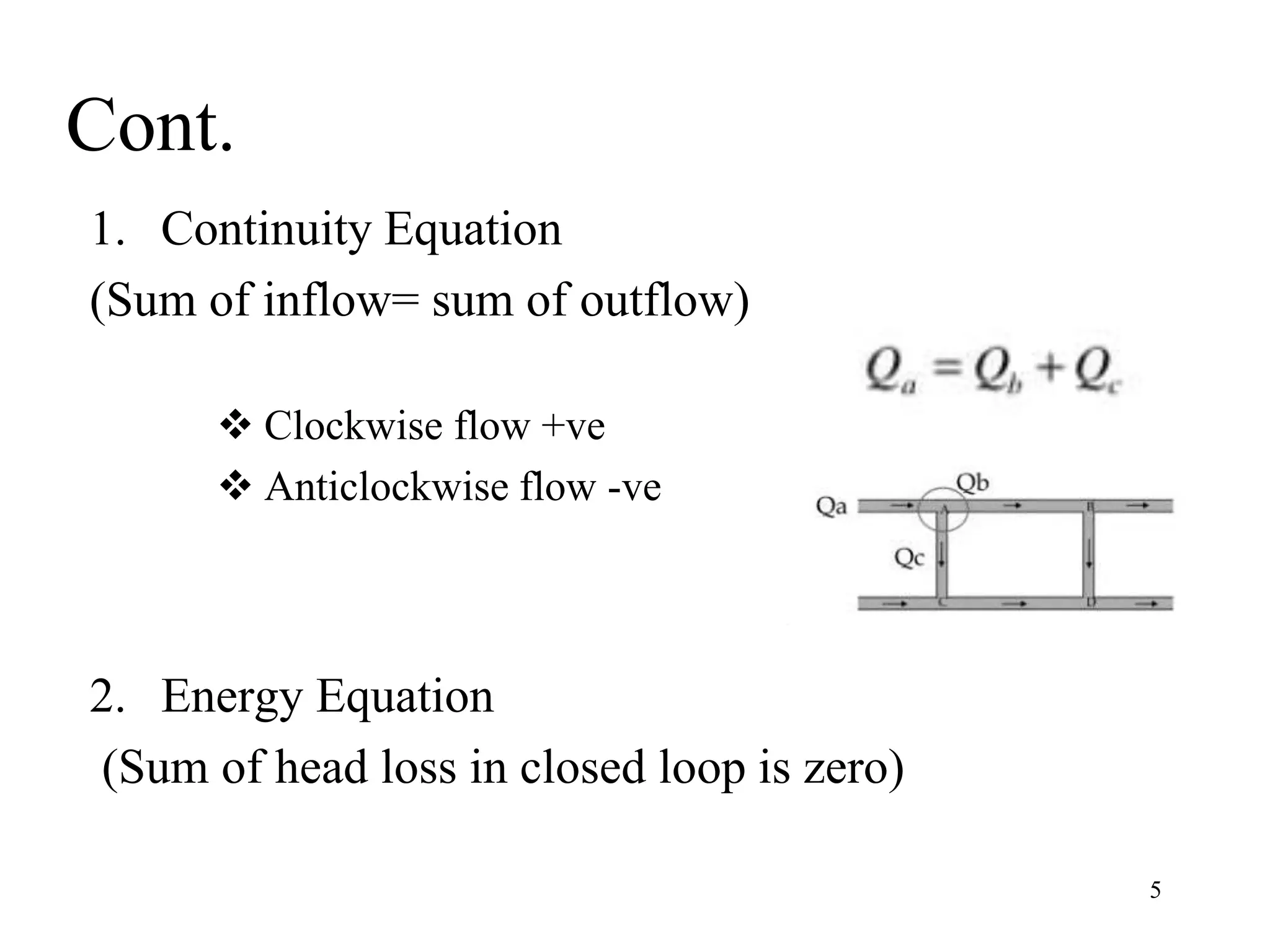
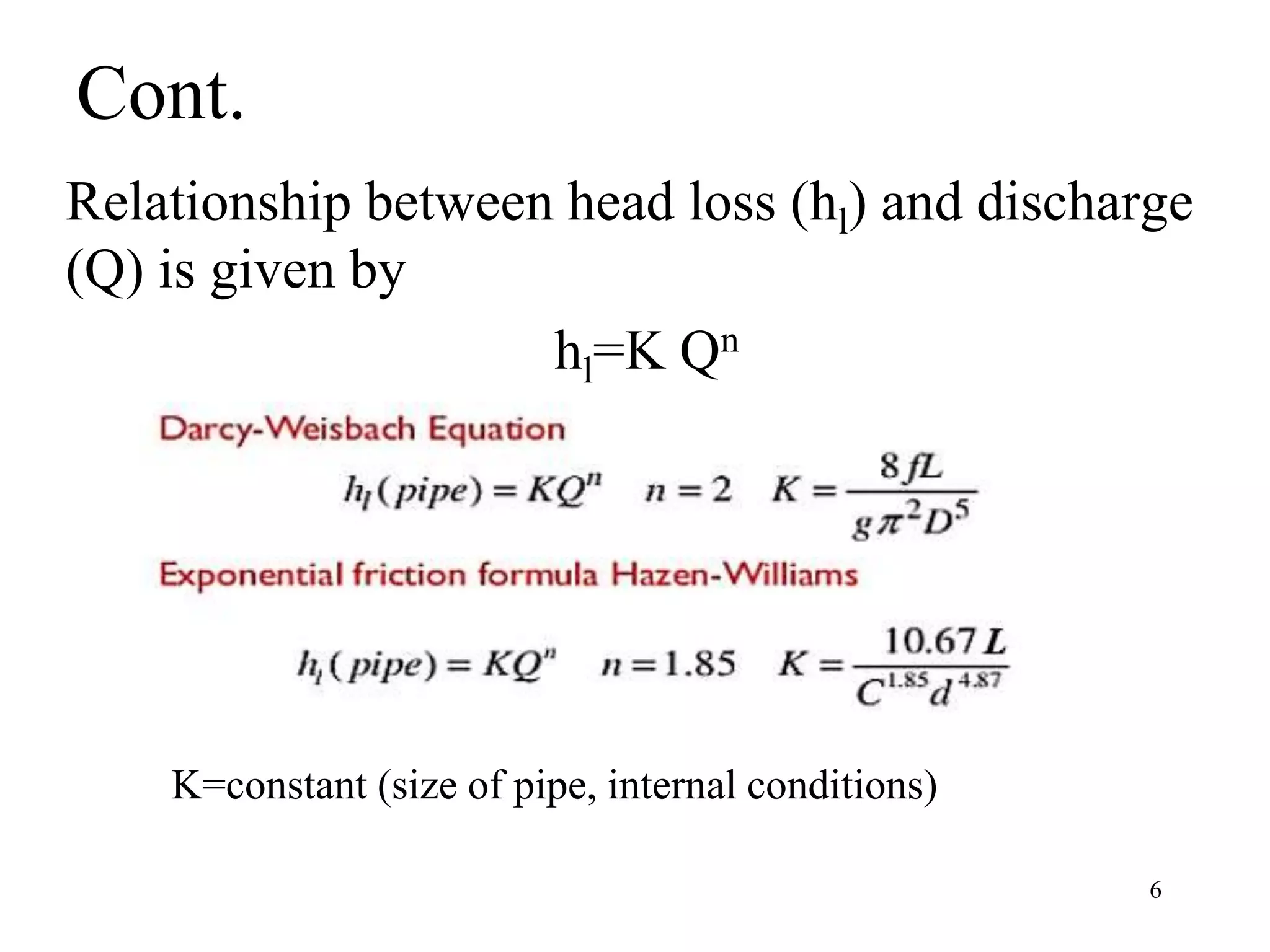
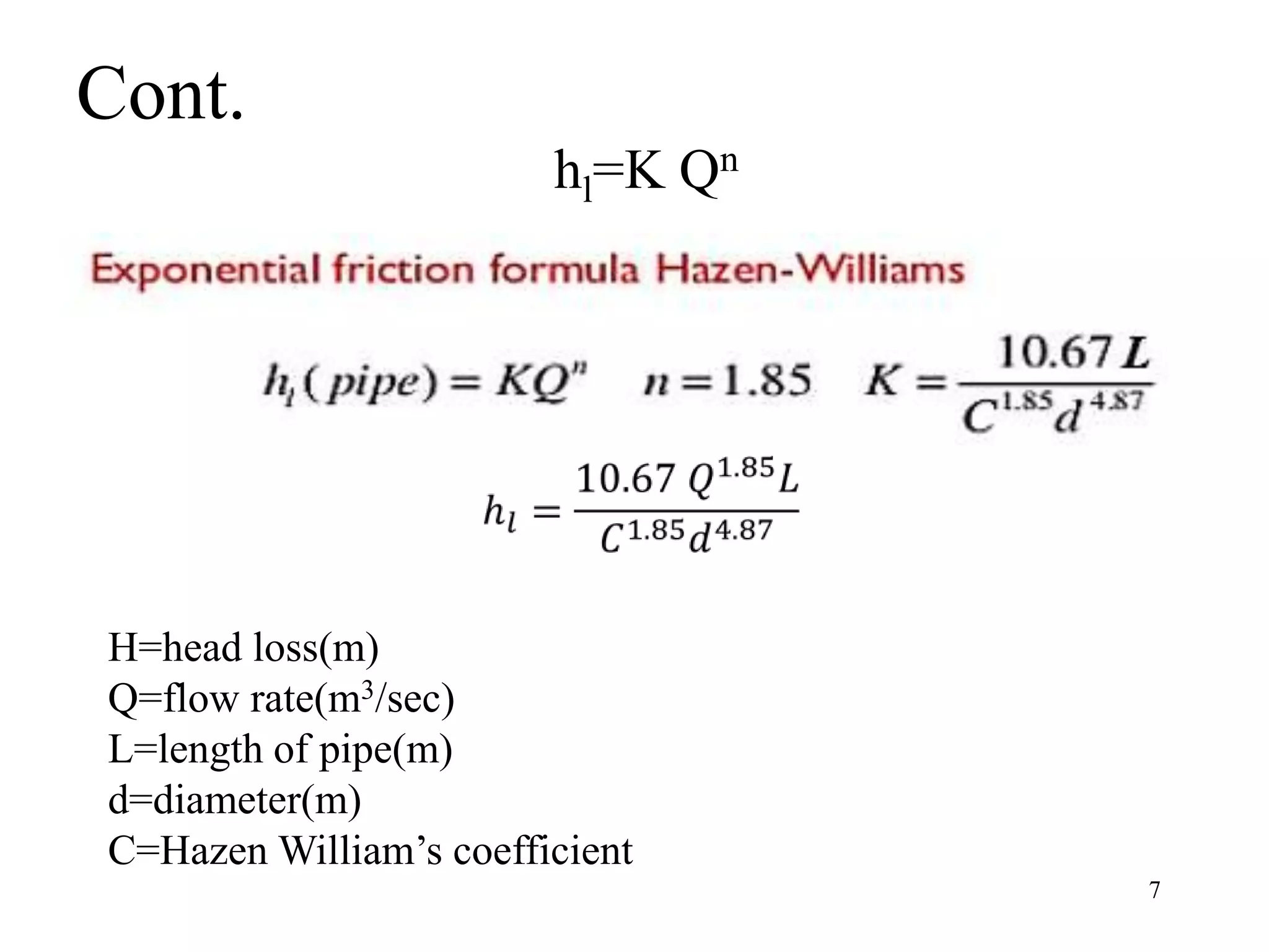
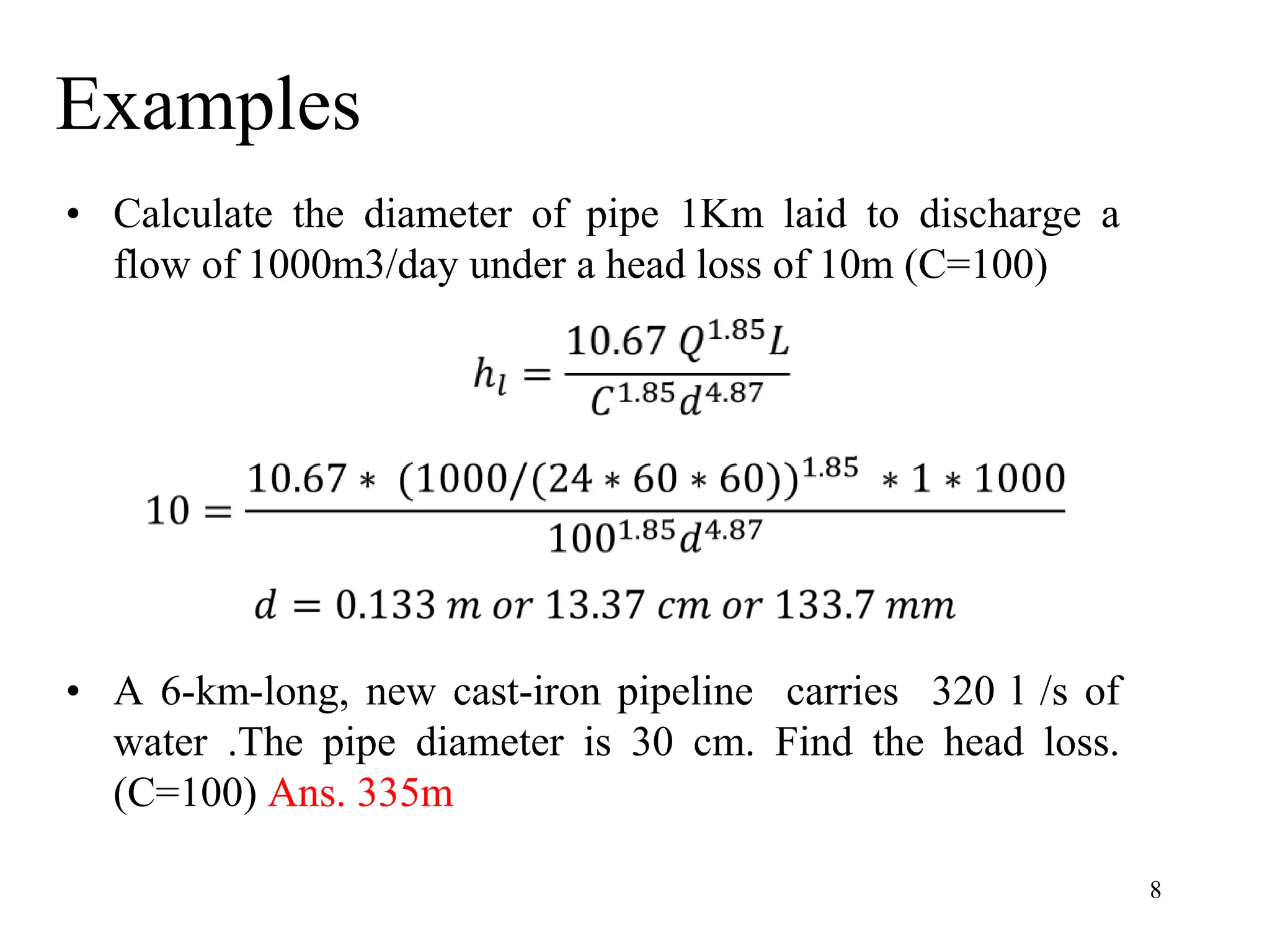
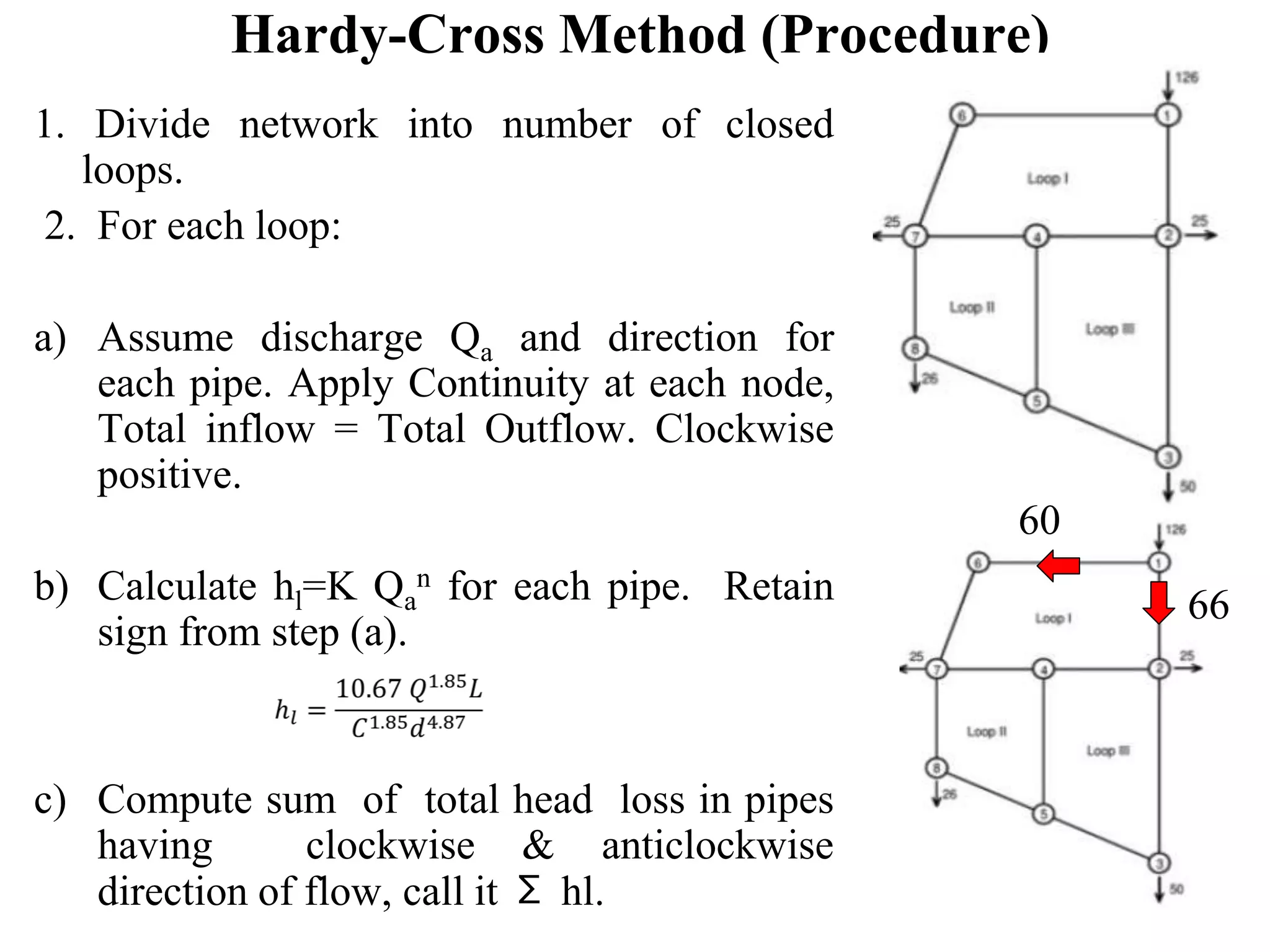
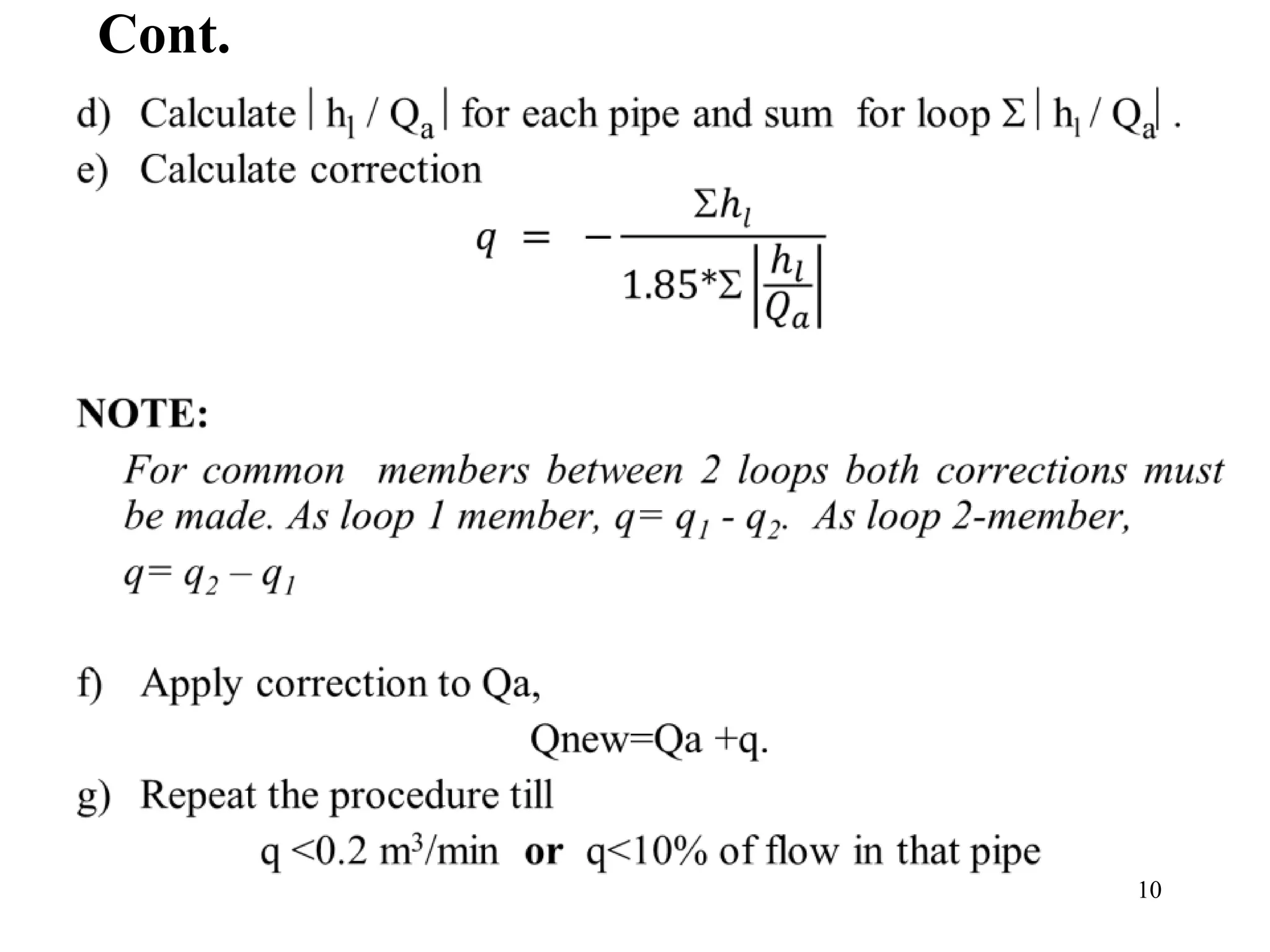
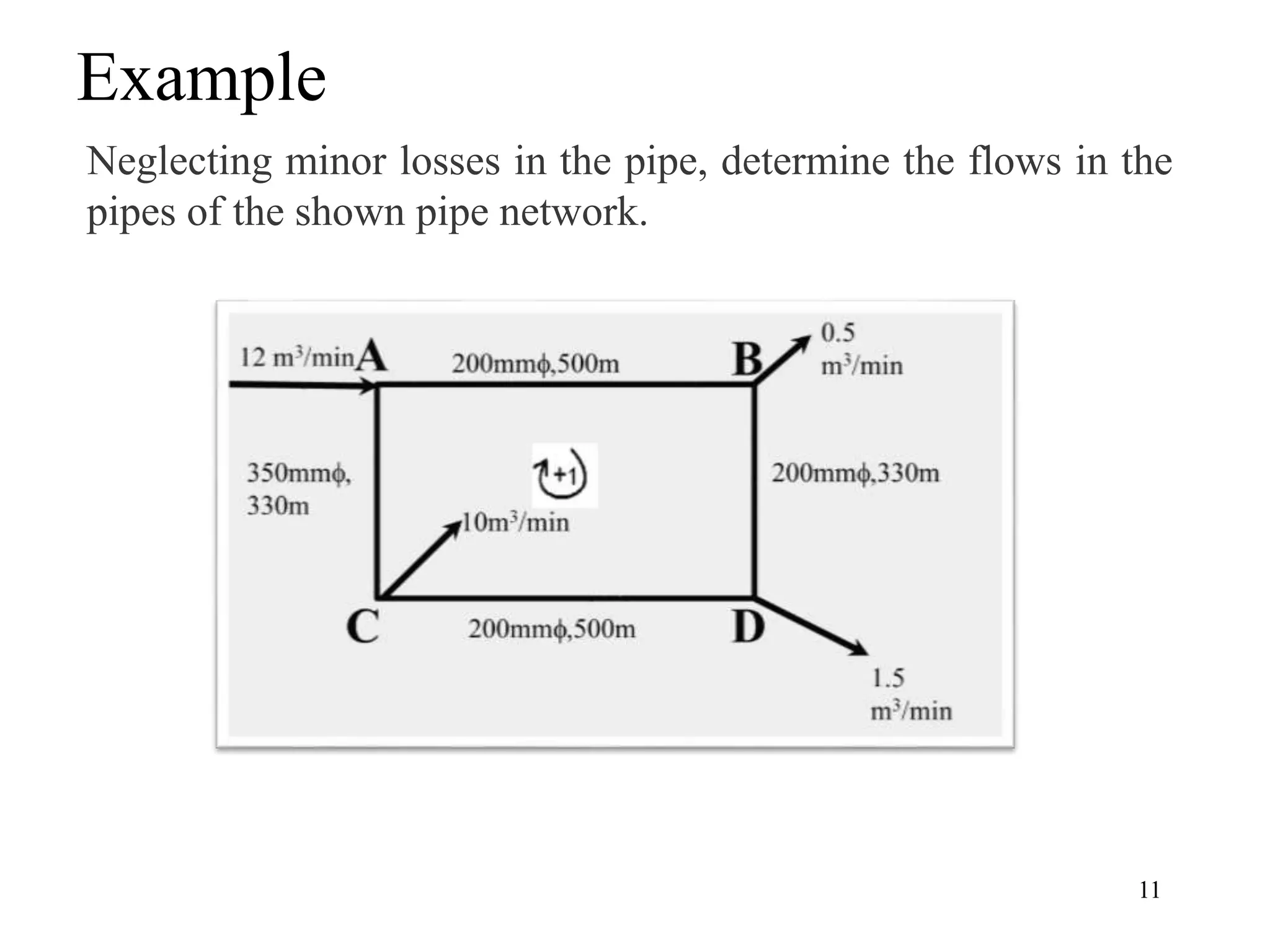
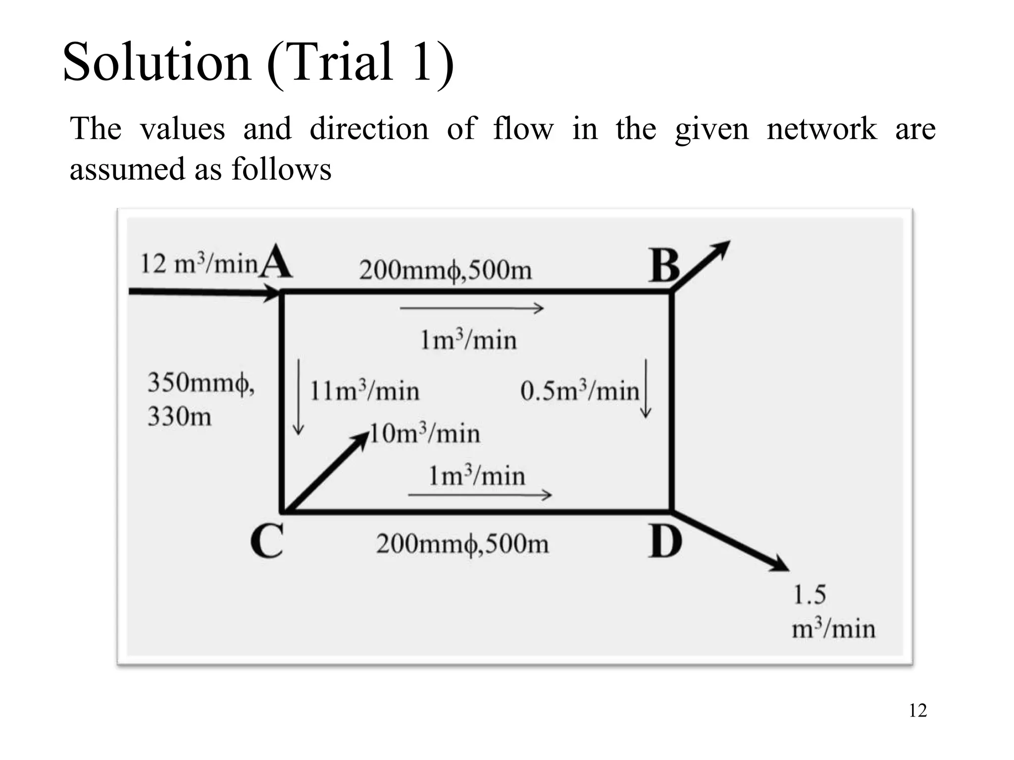
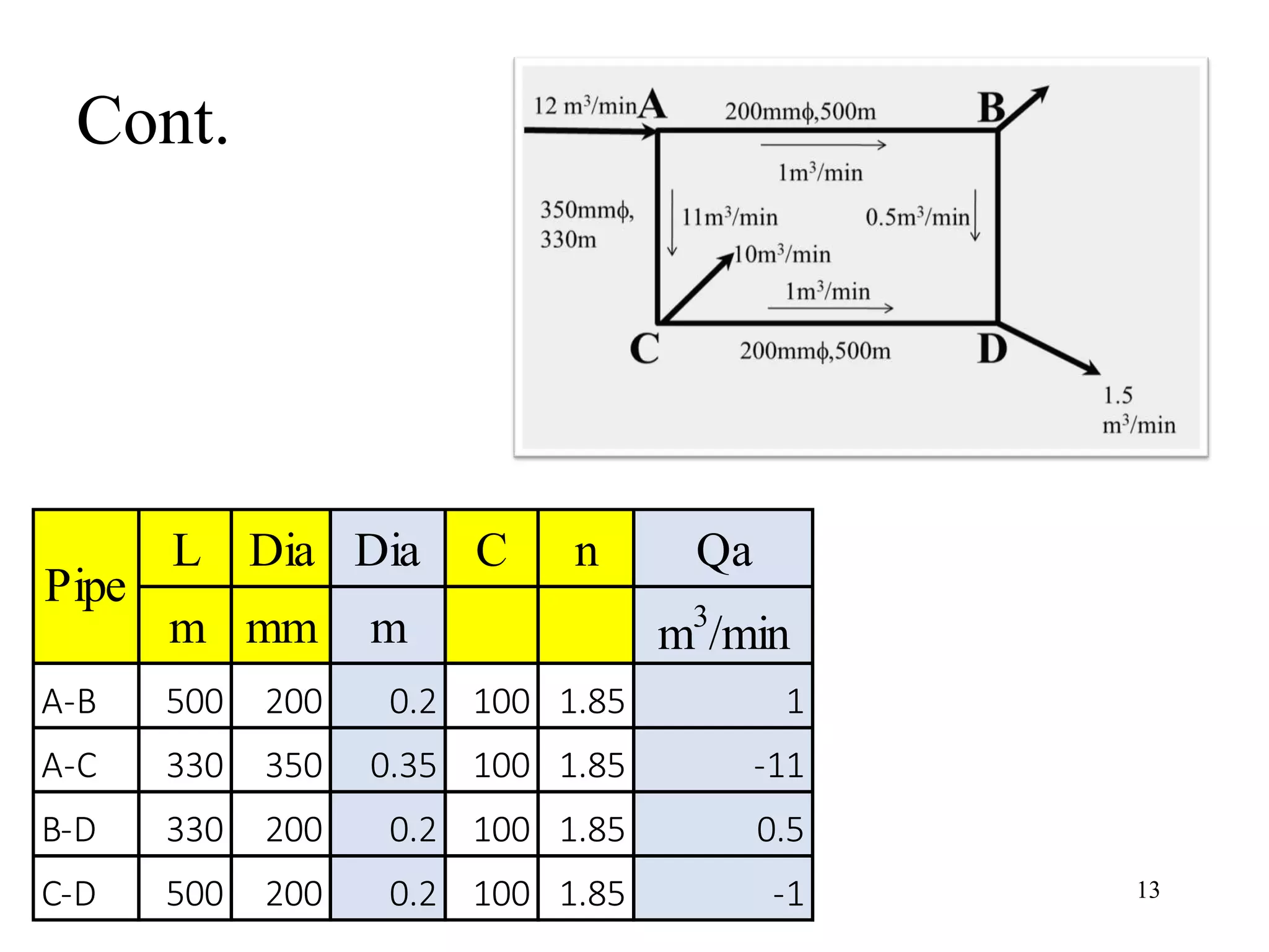
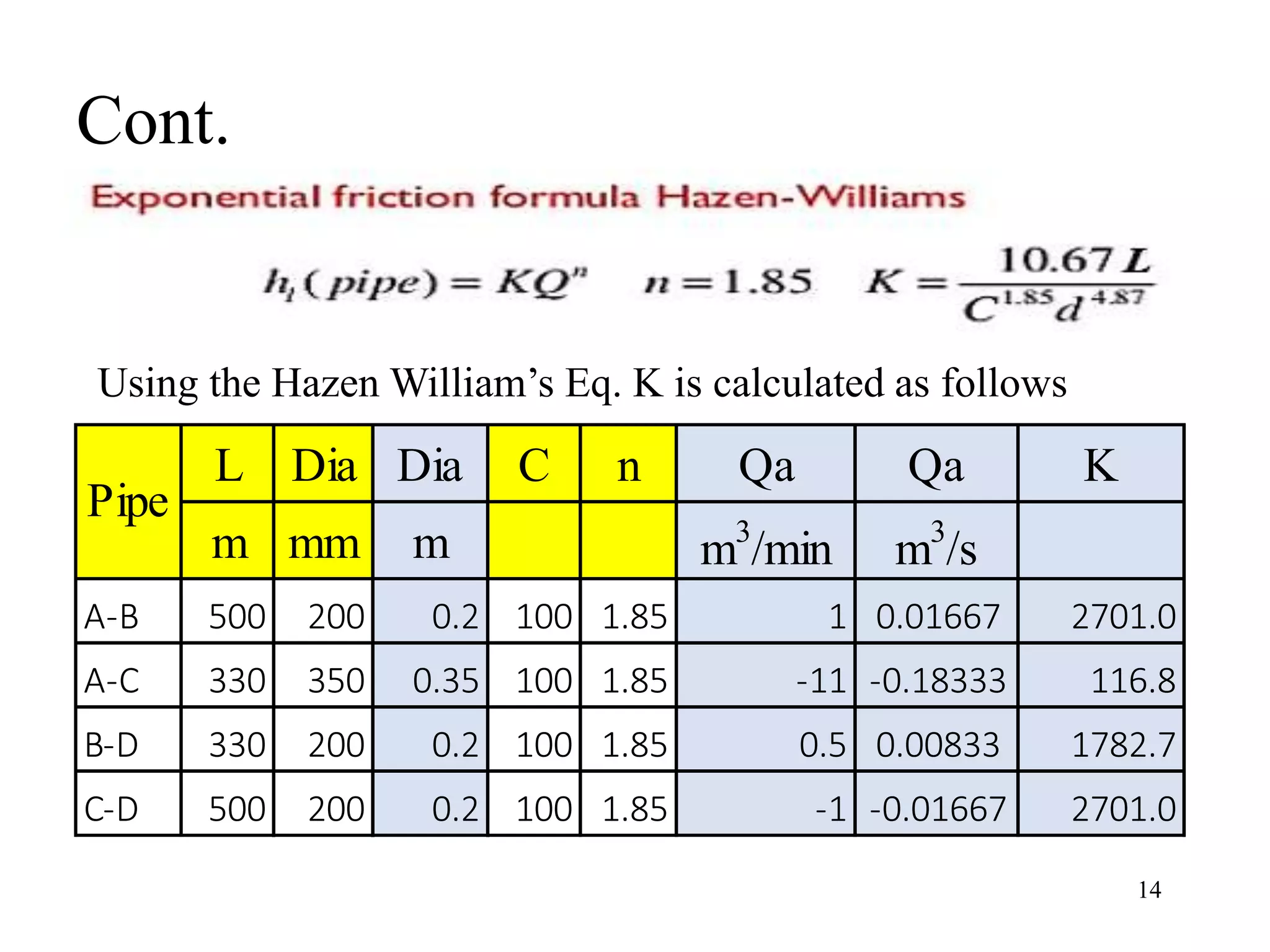
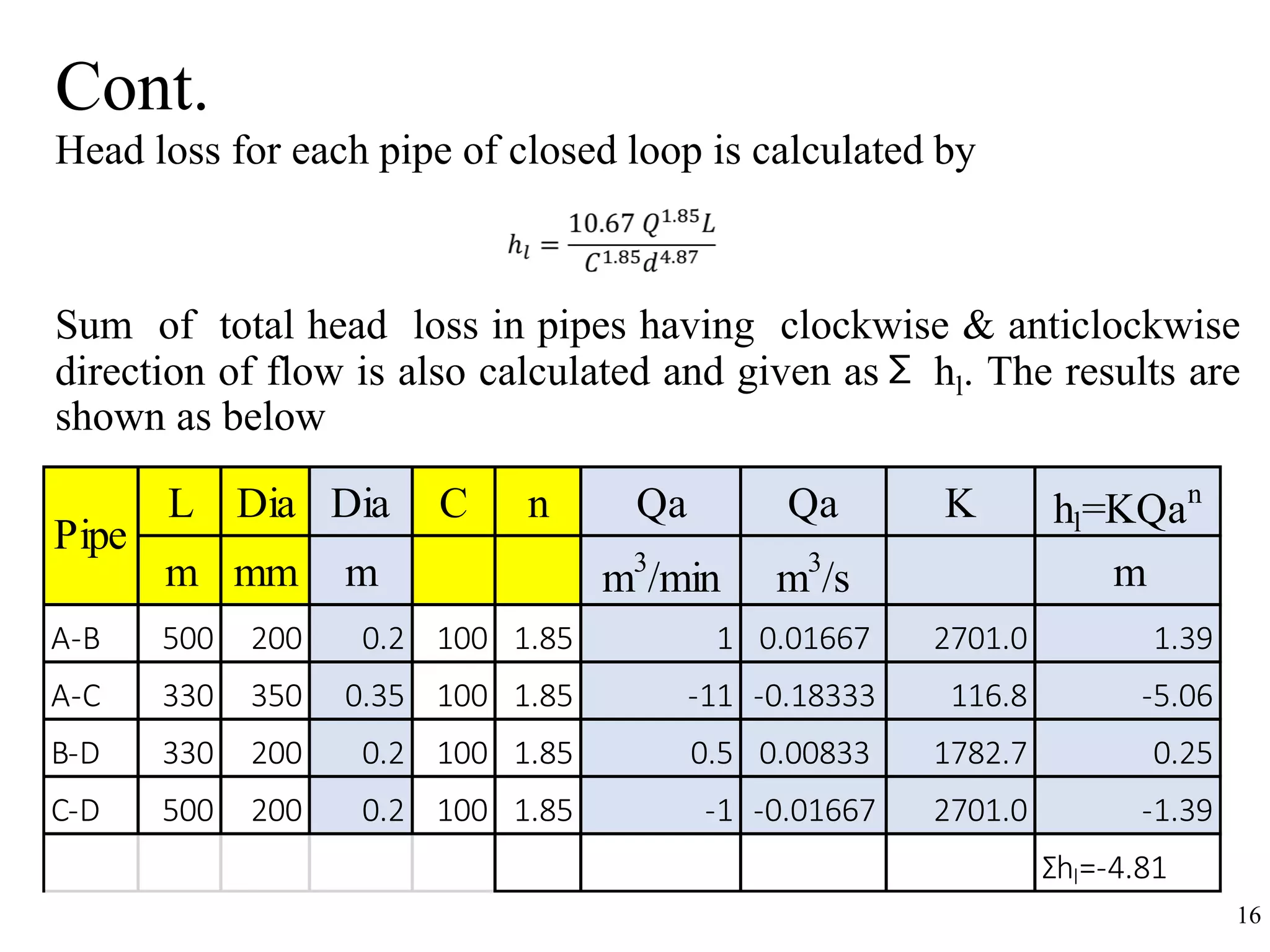
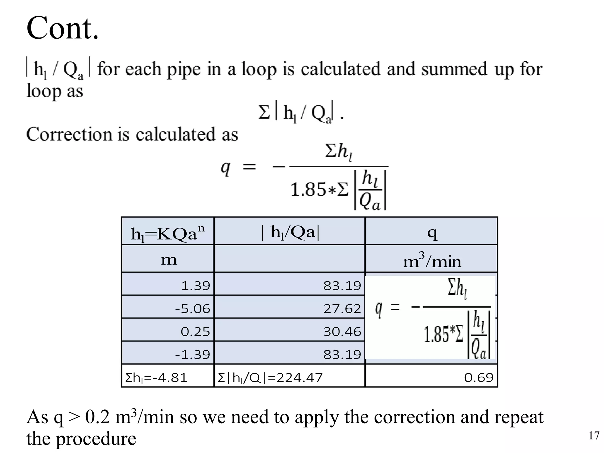
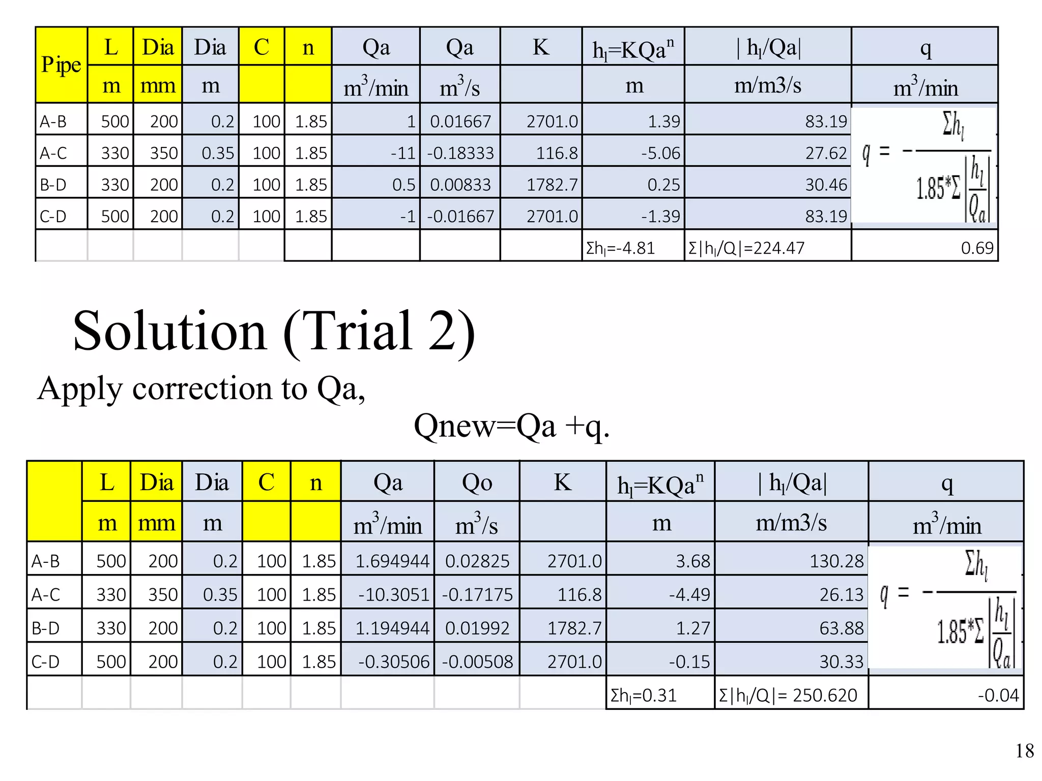
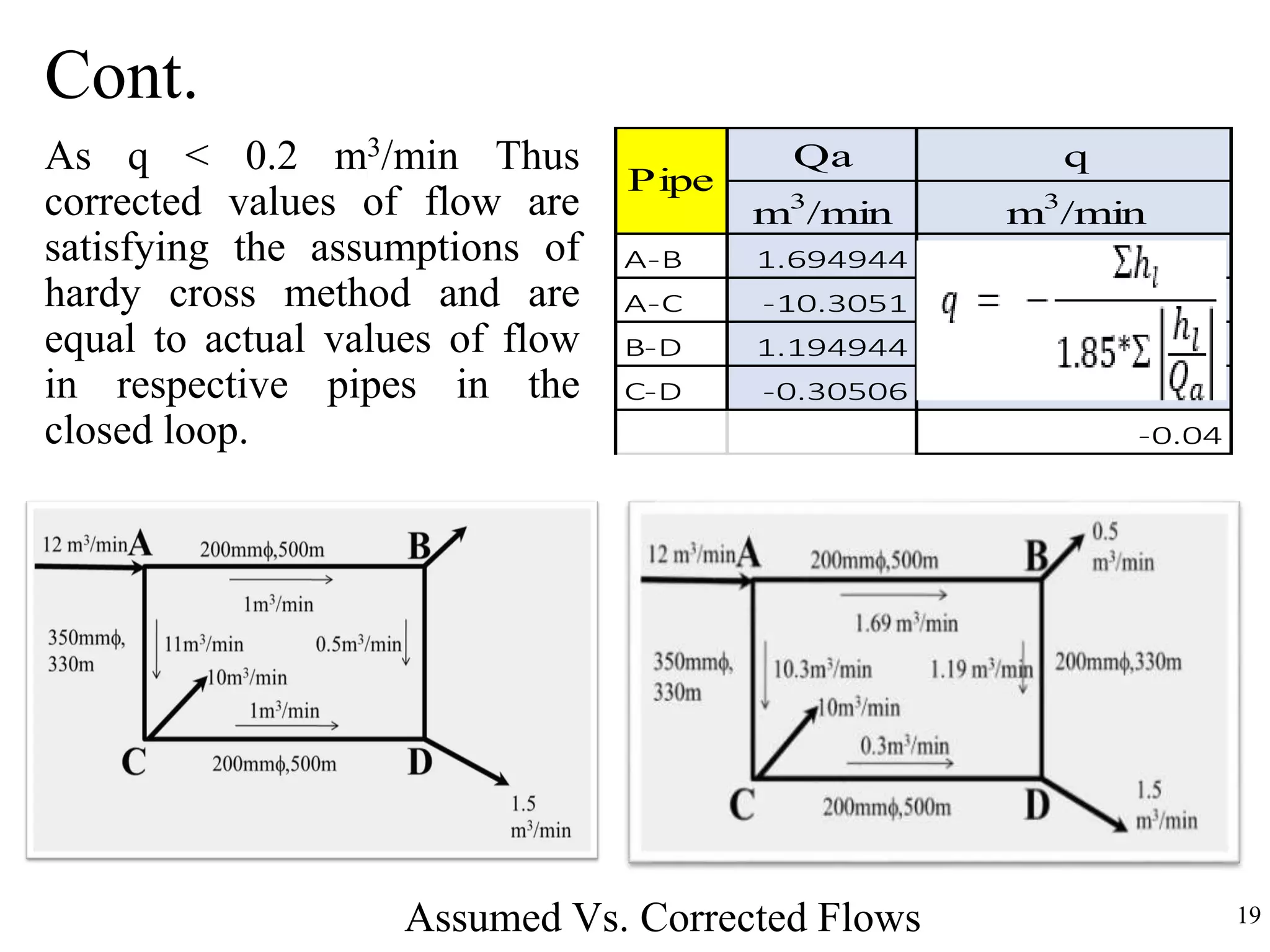
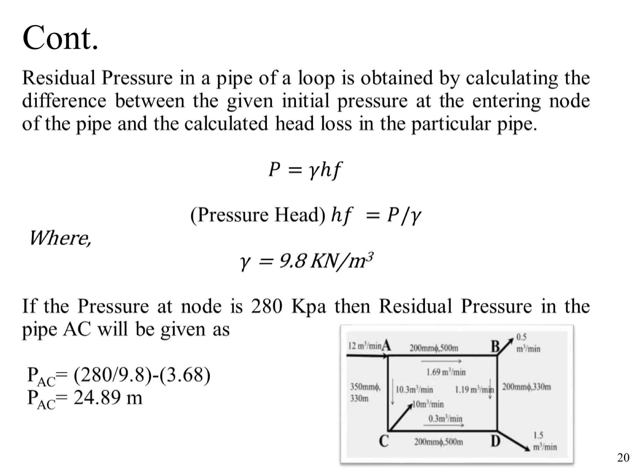
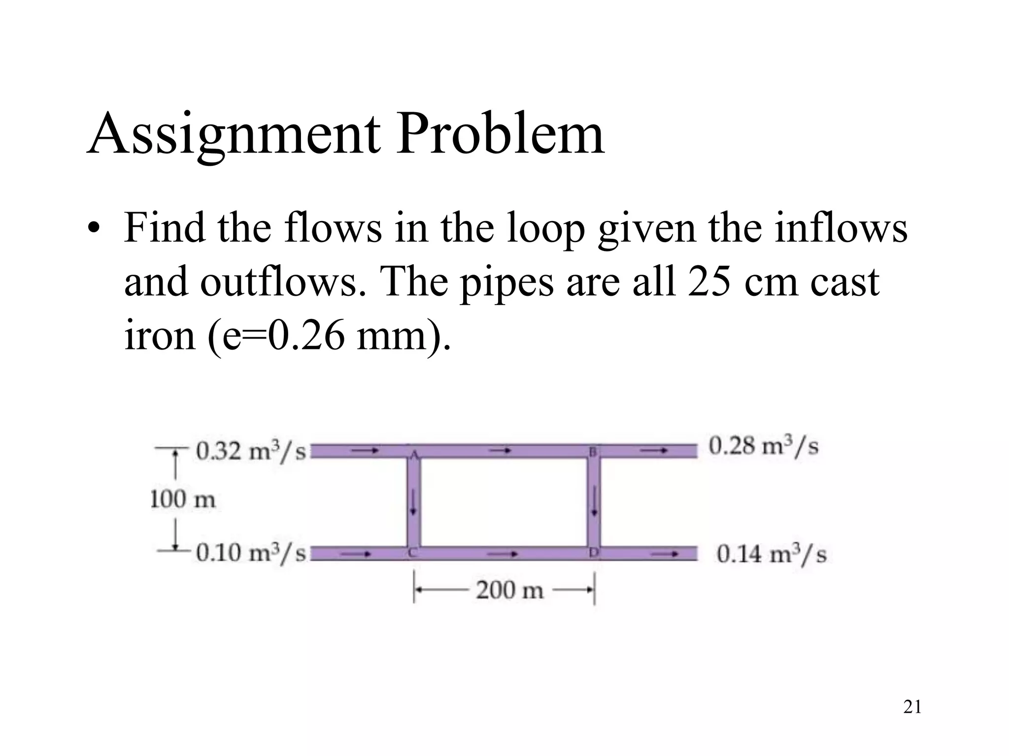
Pipe Network Analysis
Hardy Cross Method
Resource Person
Engr. Sidra Rashid
sidradar9@gmail.com
Pipe Network Analysis
It involves the investigation of the outflow
points of the network for
1. Pipe flow rates
2. Pressure heads
The flow rates and pressure heads must satisfy
the continuity and energy equations.
2
Methods of Pipe Network Analysis
1. Hardy Cross Method
2. Nodal Method
3. Newton-Raphson Method
Hardy-Cross Method is earliest systematic method of
network analysis
3
Hardy cross method
Its an iterative approach of pipe analysis
Also known as head balance or closed loop
method.
Applicable to system of pipes forming closed
loops.
• Method is based on
1. Continuity Equation
2. Energy Equation
4
Cont.
1. Continuity Equation
(Sum of inflow= sum of outflow)
 Clockwise flow +ve
 Anticlockwise flow -ve
2. Energy Equation
(Sum of head loss in closed loop is zero)
5
Cont.
Relationship between head loss (hl) and discharge
(Q) is given by
hl=K Qn
6
K=constant (size of pipe, internal conditions)
Cont.
hl=K Qn
7
H=head loss(m)
Q=flow rate(m3/sec)
L=length of pipe(m)
d=diameter(m)
C=Hazen William’s coefficient
Examples
• Calculate the diameter of pipe 1Km laid to discharge a
flow of 1000m3/day under a head loss of 10m (C=100)
• A 6-km-long, new cast-iron pipeline carries 320 l /s of
water .The pipe diameter is 30 cm. Find the head loss.
(C=100) Ans. 335m
8
Hardy-Cross Method (Procedure)
1. Divide network into number of closed
loops.
2. For each loop:
a) Assume discharge Qa and direction for
each pipe. Apply Continuity at each node,
Total inflow = Total Outflow. Clockwise
positive.
b) Calculate hl=K Qa
n for each pipe. Retain
sign from step (a).
c) Compute sum of total head loss in pipes
having clockwise & anticlockwise
direction of flow, call it Σ hl. 9
60
66
Cont.
10
Example
11
Neglecting minor losses in the pipe, determine the flows in the
pipes of the shown pipe network.
Solution (Trial 1)
12
The values and direction of flow in the given network are
assumed as follows
Cont.
13
L Dia Dia C n Qa
m mm m m3
/min
A-B 500 200 0.2 100 1.85 1
A-C 330 350 0.35 100 1.85 -11
B-D 330 200 0.2 100 1.85 0.5
C-D 500 200 0.2 100 1.85 -1
Pipe
Cont.
14
Using the Hazen William’s Eq. K is calculated as follows
L Dia Dia C n Qa Qa K
m mm m m3
/min m3
/s
A-B 500 200 0.2 100 1.85 1 0.01667 2701.0
A-C 330 350 0.35 100 1.85 -11 -0.18333 116.8
B-D 330 200 0.2 100 1.85 0.5 0.00833 1782.7
C-D 500 200 0.2 100 1.85 -1 -0.01667 2701.0
Pipe
Cont.
15
Using the Hazen William’s Eq. K is calculated as follows
L Dia Dia C n Qa Qa K
m mm m m3
/min m3
/s
A-B 500 200 0.2 100 1.85 1 0.01667 2701.0
A-C 330 350 0.35 100 1.85 -11 -0.18333 116.8
B-D 330 200 0.2 100 1.85 0.5 0.00833 1782.7
C-D 500 200 0.2 100 1.85 -1 -0.01667 2701.0
Pipe
Cont.
16
Head loss for each pipe of closed loop is calculated by
Sum of total head loss in pipes having clockwise & anticlockwise
direction of flow is also calculated and given asΣ hl. The results are
shown as below
L Dia Dia C n Qa Qa K hl=KQan
m mm m m3
/min m3
/s m
A-B 500 200 0.2 100 1.85 1 0.01667 2701.0 1.39
A-C 330 350 0.35 100 1.85 -11 -0.18333 116.8 -5.06
B-D 330 200 0.2 100 1.85 0.5 0.00833 1782.7 0.25
C-D 500 200 0.2 100 1.85 -1 -0.01667 2701.0 -1.39
Σhl=-4.81
Pipe
Cont.
17
hl=KQan | hl/Qa| q
m m3
/min
1.39 83.19
-5.06 27.62
0.25 30.46
-1.39 83.19
Σhl=-4.81 Σ|hl/Q|=224.47 0.69
As q > 0.2 m3/min so we need to apply the correction and repeat
the procedure
Solution (Trial 2)
18
L Dia Dia C n Qa Qa K hl=KQan | hl/Qa| q
m mm m m3
/min m3
/s m m/m3/s m3
/min
A-B 500 200 0.2 100 1.85 1 0.01667 2701.0 1.39 83.19
A-C 330 350 0.35 100 1.85 -11 -0.18333 116.8 -5.06 27.62
B-D 330 200 0.2 100 1.85 0.5 0.00833 1782.7 0.25 30.46
C-D 500 200 0.2 100 1.85 -1 -0.01667 2701.0 -1.39 83.19
Σhl=-4.81 Σ|hl/Q|=224.47 0.69
Pipe
Apply correction to Qa,
Qnew=Qa +q.
L Dia Dia C n Qa Qo K hl=KQan | hl/Qa| q
m mm m m3
/min m3
/s m m/m3/s m3
/min
A-B 500 200 0.2 100 1.85 1.694944 0.02825 2701.0 3.68 130.28
A-C 330 350 0.35 100 1.85 -10.3051 -0.17175 116.8 -4.49 26.13
B-D 330 200 0.2 100 1.85 1.194944 0.01992 1782.7 1.27 63.88
C-D 500 200 0.2 100 1.85 -0.30506 -0.00508 2701.0 -0.15 30.33
Σhl=0.31 Σ|hl/Q|= 250.620 -0.04
Cont.
19
As q < 0.2 m3/min Thus
corrected values of flow are
satisfying the assumptions of
hardy cross method and are
equal to actual values of flow
in respective pipes in the
closed loop.
Qa q
m3
/min m3
/min
A-B 1.694944
A-C -10.3051
B-D 1.194944
C-D -0.30506
-0.04
Pipe
Assumed Vs. Corrected Flows
Cont.
20
Assignment Problem
• Find the flows in the loop given the inflows
and outflows. The pipes are all 25 cm cast
iron (e=0.26 mm).
21

Hardy cross method of pipe network analysis

  • 1.
    Pipe Network Analysis HardyCross Method Resource Person Engr. Sidra Rashid sidradar9@gmail.com
  • 2.
    Pipe Network Analysis Itinvolves the investigation of the outflow points of the network for 1. Pipe flow rates 2. Pressure heads The flow rates and pressure heads must satisfy the continuity and energy equations. 2
  • 3.
    Methods of PipeNetwork Analysis 1. Hardy Cross Method 2. Nodal Method 3. Newton-Raphson Method Hardy-Cross Method is earliest systematic method of network analysis 3
  • 4.
    Hardy cross method Itsan iterative approach of pipe analysis Also known as head balance or closed loop method. Applicable to system of pipes forming closed loops. • Method is based on 1. Continuity Equation 2. Energy Equation 4
  • 5.
    Cont. 1. Continuity Equation (Sumof inflow= sum of outflow)  Clockwise flow +ve  Anticlockwise flow -ve 2. Energy Equation (Sum of head loss in closed loop is zero) 5
  • 6.
    Cont. Relationship between headloss (hl) and discharge (Q) is given by hl=K Qn 6 K=constant (size of pipe, internal conditions)
  • 7.
    Cont. hl=K Qn 7 H=head loss(m) Q=flowrate(m3/sec) L=length of pipe(m) d=diameter(m) C=Hazen William’s coefficient
  • 8.
    Examples • Calculate thediameter of pipe 1Km laid to discharge a flow of 1000m3/day under a head loss of 10m (C=100) • A 6-km-long, new cast-iron pipeline carries 320 l /s of water .The pipe diameter is 30 cm. Find the head loss. (C=100) Ans. 335m 8
  • 9.
    Hardy-Cross Method (Procedure) 1.Divide network into number of closed loops. 2. For each loop: a) Assume discharge Qa and direction for each pipe. Apply Continuity at each node, Total inflow = Total Outflow. Clockwise positive. b) Calculate hl=K Qa n for each pipe. Retain sign from step (a). c) Compute sum of total head loss in pipes having clockwise & anticlockwise direction of flow, call it Σ hl. 9 60 66
  • 10.
  • 11.
    Example 11 Neglecting minor lossesin the pipe, determine the flows in the pipes of the shown pipe network.
  • 12.
    Solution (Trial 1) 12 Thevalues and direction of flow in the given network are assumed as follows
  • 13.
    Cont. 13 L Dia DiaC n Qa m mm m m3 /min A-B 500 200 0.2 100 1.85 1 A-C 330 350 0.35 100 1.85 -11 B-D 330 200 0.2 100 1.85 0.5 C-D 500 200 0.2 100 1.85 -1 Pipe
  • 14.
    Cont. 14 Using the HazenWilliam’s Eq. K is calculated as follows L Dia Dia C n Qa Qa K m mm m m3 /min m3 /s A-B 500 200 0.2 100 1.85 1 0.01667 2701.0 A-C 330 350 0.35 100 1.85 -11 -0.18333 116.8 B-D 330 200 0.2 100 1.85 0.5 0.00833 1782.7 C-D 500 200 0.2 100 1.85 -1 -0.01667 2701.0 Pipe
  • 15.
    Cont. 15 Using the HazenWilliam’s Eq. K is calculated as follows L Dia Dia C n Qa Qa K m mm m m3 /min m3 /s A-B 500 200 0.2 100 1.85 1 0.01667 2701.0 A-C 330 350 0.35 100 1.85 -11 -0.18333 116.8 B-D 330 200 0.2 100 1.85 0.5 0.00833 1782.7 C-D 500 200 0.2 100 1.85 -1 -0.01667 2701.0 Pipe
  • 16.
    Cont. 16 Head loss foreach pipe of closed loop is calculated by Sum of total head loss in pipes having clockwise & anticlockwise direction of flow is also calculated and given asΣ hl. The results are shown as below L Dia Dia C n Qa Qa K hl=KQan m mm m m3 /min m3 /s m A-B 500 200 0.2 100 1.85 1 0.01667 2701.0 1.39 A-C 330 350 0.35 100 1.85 -11 -0.18333 116.8 -5.06 B-D 330 200 0.2 100 1.85 0.5 0.00833 1782.7 0.25 C-D 500 200 0.2 100 1.85 -1 -0.01667 2701.0 -1.39 Σhl=-4.81 Pipe
  • 17.
    Cont. 17 hl=KQan | hl/Qa|q m m3 /min 1.39 83.19 -5.06 27.62 0.25 30.46 -1.39 83.19 Σhl=-4.81 Σ|hl/Q|=224.47 0.69 As q > 0.2 m3/min so we need to apply the correction and repeat the procedure
  • 18.
    Solution (Trial 2) 18 LDia Dia C n Qa Qa K hl=KQan | hl/Qa| q m mm m m3 /min m3 /s m m/m3/s m3 /min A-B 500 200 0.2 100 1.85 1 0.01667 2701.0 1.39 83.19 A-C 330 350 0.35 100 1.85 -11 -0.18333 116.8 -5.06 27.62 B-D 330 200 0.2 100 1.85 0.5 0.00833 1782.7 0.25 30.46 C-D 500 200 0.2 100 1.85 -1 -0.01667 2701.0 -1.39 83.19 Σhl=-4.81 Σ|hl/Q|=224.47 0.69 Pipe Apply correction to Qa, Qnew=Qa +q. L Dia Dia C n Qa Qo K hl=KQan | hl/Qa| q m mm m m3 /min m3 /s m m/m3/s m3 /min A-B 500 200 0.2 100 1.85 1.694944 0.02825 2701.0 3.68 130.28 A-C 330 350 0.35 100 1.85 -10.3051 -0.17175 116.8 -4.49 26.13 B-D 330 200 0.2 100 1.85 1.194944 0.01992 1782.7 1.27 63.88 C-D 500 200 0.2 100 1.85 -0.30506 -0.00508 2701.0 -0.15 30.33 Σhl=0.31 Σ|hl/Q|= 250.620 -0.04
  • 19.
    Cont. 19 As q <0.2 m3/min Thus corrected values of flow are satisfying the assumptions of hardy cross method and are equal to actual values of flow in respective pipes in the closed loop. Qa q m3 /min m3 /min A-B 1.694944 A-C -10.3051 B-D 1.194944 C-D -0.30506 -0.04 Pipe Assumed Vs. Corrected Flows
  • 20.
  • 21.
    Assignment Problem • Findthe flows in the loop given the inflows and outflows. The pipes are all 25 cm cast iron (e=0.26 mm). 21