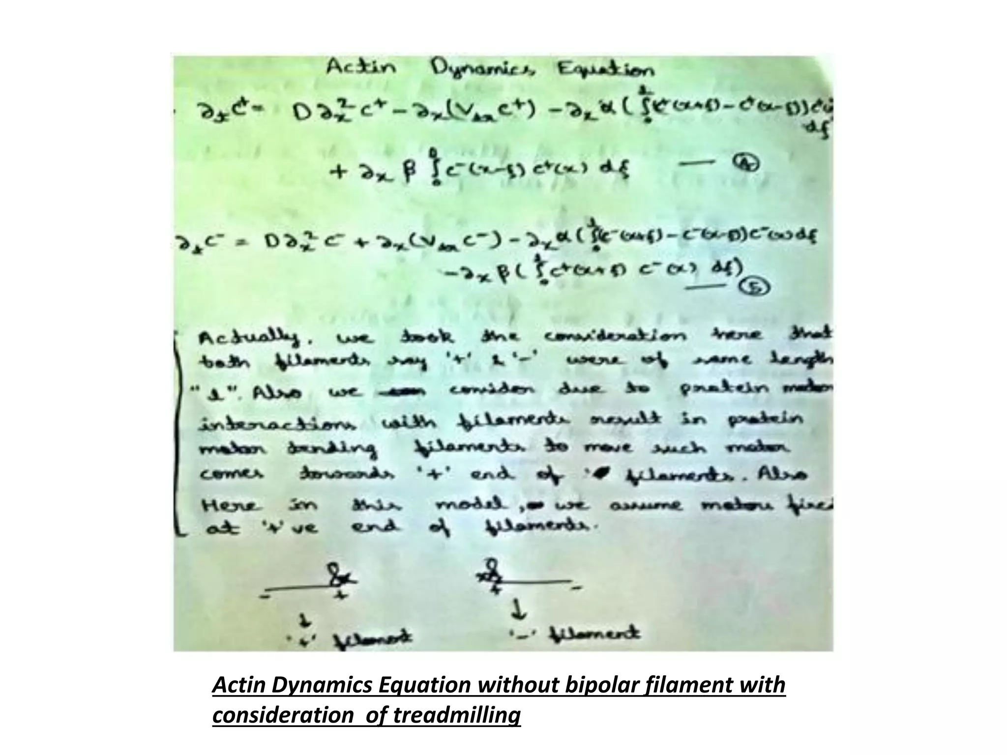
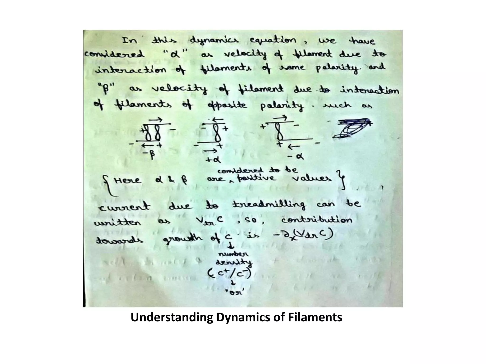
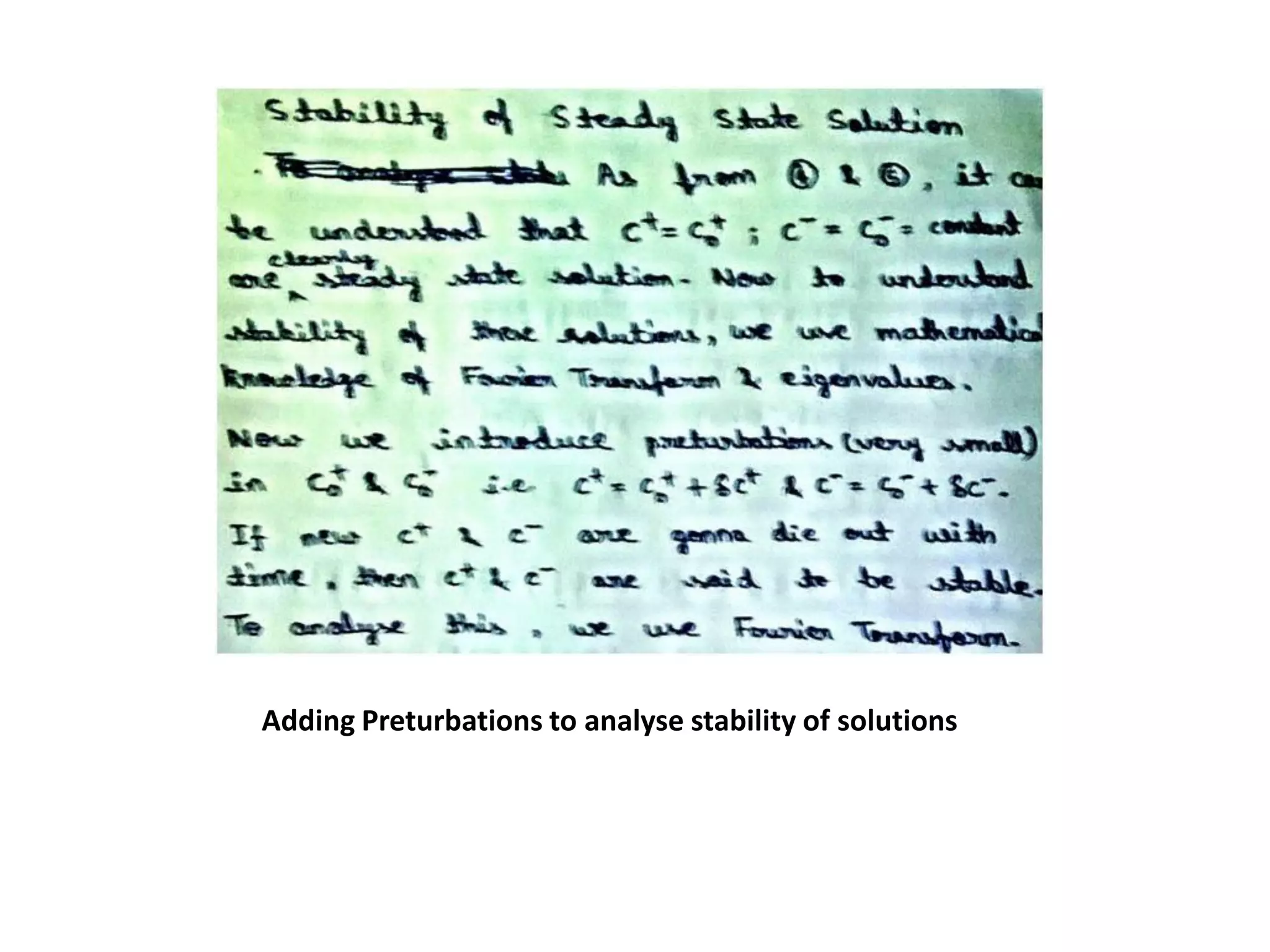
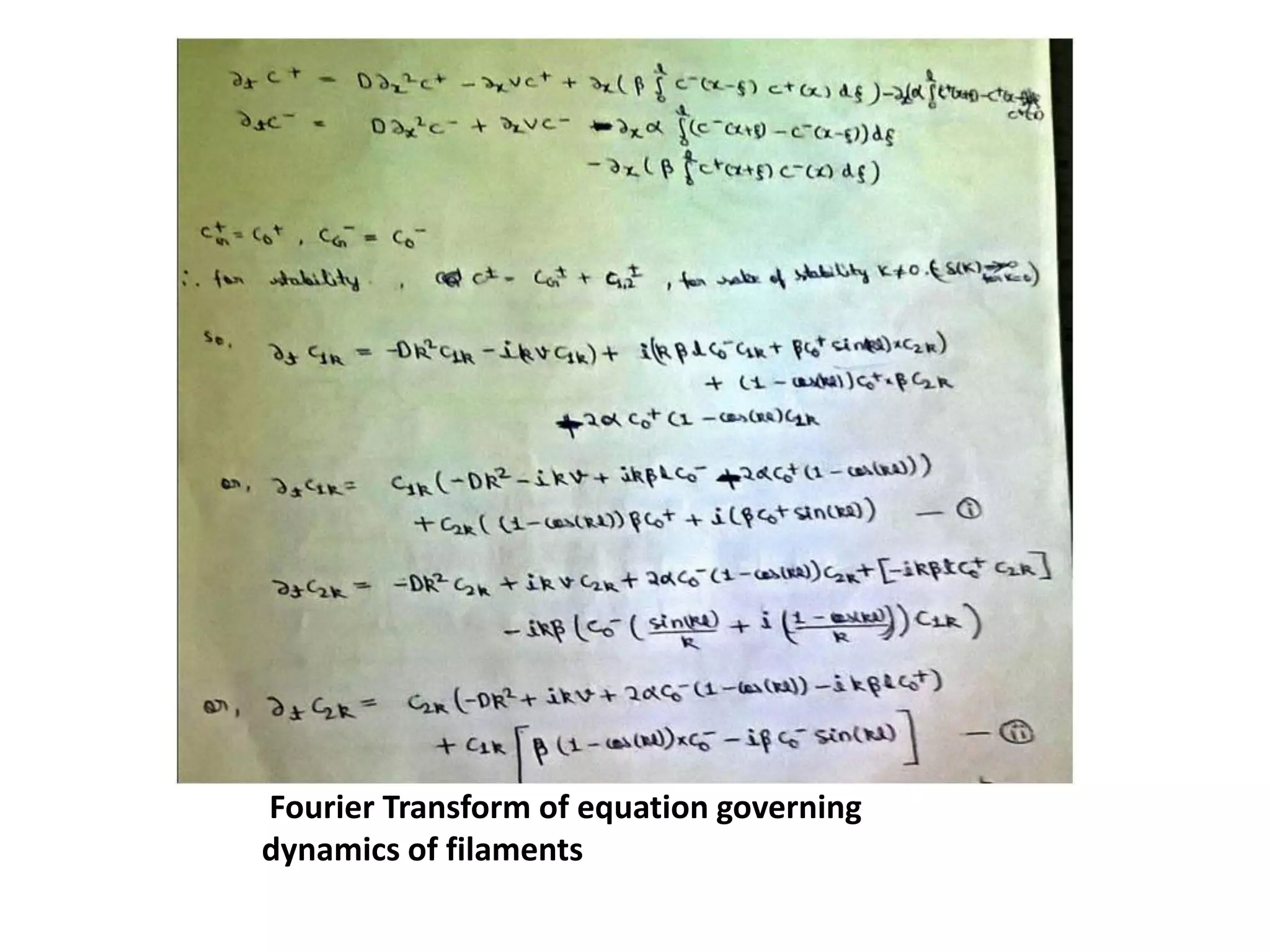
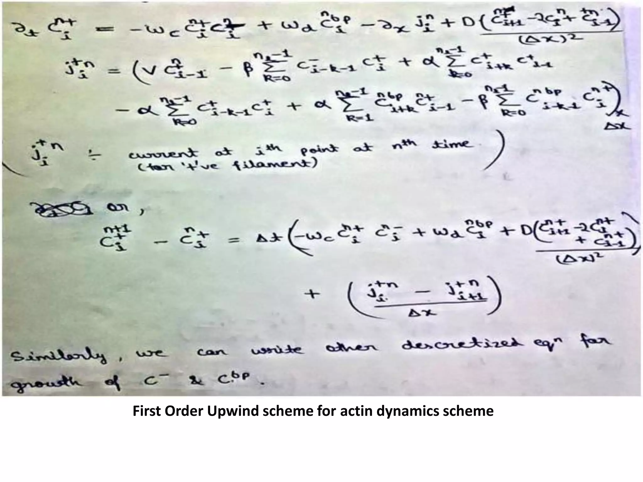
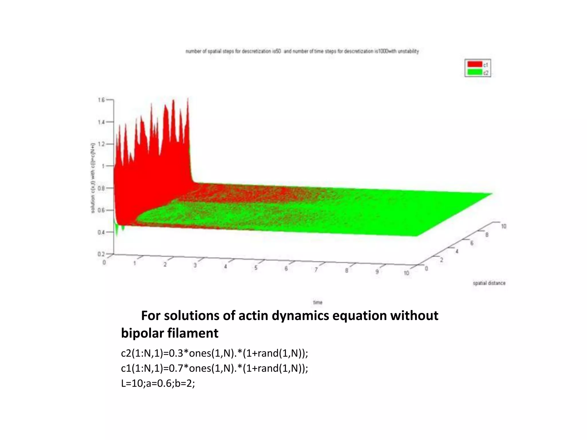
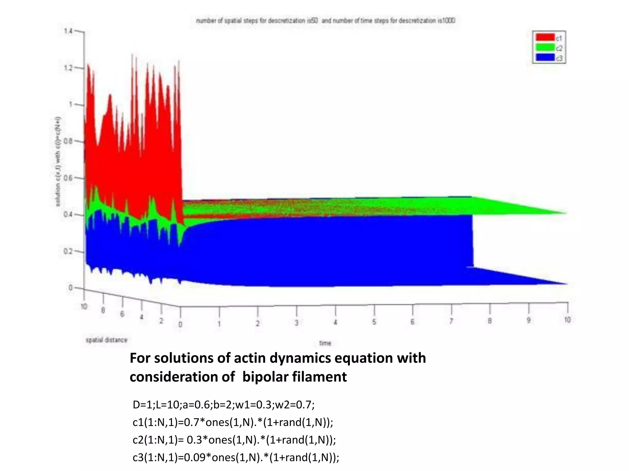
This document is a summer internship report submitted by Prafull Kumar Sharma to Karsten Kruse at the University of Saarland in Germany. It summarizes Prafull's work analyzing the dynamics of actin filaments in the contractile ring numerically. Prafull first learned techniques for numerically solving diffusion equations. He then analyzed models of actin filament dynamics both without and with bipolar filaments, studying stability and performing simulations. Key results included verifying that stability only depends on the wavenumber k=2pi/L. Prafull gained experience with programming in MATLAB and solving nonlinear equations during the productive internship.

1. DYNAMICS OF ACTIN FILAMENTS IN
THE CONTRACTILE RING
Summer Internship Report
Submitted to:
Bio-Physics Group, AG Karsten Kruse
University of Saarland , Germany
Submitted by:
Prafull Kumar Sharma
2nd year undergraduate B.Tech .(Engineering Physics)
Indian Institute of Technology (Delhi), India

2. Numerical Analysis of Diffusion
equation
• First I was supposed to learn basic techniques used in
numerical analysis to analyse solutions of a diffusion
equation.We use Numerical Analysis to understand the
behaviour of solution of the equations involved in our
project.To begin with ,I solved 1-D diffusion equation using
backward euler and forwad euler method algorithms to
show on computer.I have used MATLAB to show solutions
for the equation.Here are some screenshots of theoretical
methods and equations involved.In the screenshots,I have
solved diffusion equation analytically with initial condition
as dirac delta function.Solution is a gaussian distribution as
expected theoretically when solved numerically on
MATLAB.

3. Solution of 1D diffusion equation using delta function
as initial condition
Gaussian Distribution as expected with theoretical analysis

4. Diffusion Equation and it’s analytical solution with
initial condition (c(x,0)) as “dirac delta function”

5. Theory Behind Forward Euler Method

6. Theoretical explanation behind Backward Euler Method

7. Numerical Analysis of Dynamics of
actin filaments without considering
Bipolar Filament
• After Basic Numerical analysis techniques,I was supposed to
analyse dynamics of actin filaments as described in “Actively
Contracting Bundles of Polar Filaments” by K.Kruse && F. Jullicher,
published in Physical Review Letters Volume 85,Number 8.
• In this Model, we consider (with our theoretical considerations) we
try to capture essential features of the ring dynamics, such as,
filament polarity, interaction between filaments through protein
motors. Here we assume that actin filaments align with perimeter
of ring. We denote the co-ordinate along the ring perimeter by x
and describe the distribution of (polar) actin filaments with respect
to x coordinates by the densities c+ (x,t) for filaments with their
plus-end pointing clockwise and c- (x,t) for filaments of the opposite
orientation. Here are some screenshots of Theoretical explanations
and equations involved.

8. Actin Dynamics Equation without bipolar filament with
consideration of treadmilling

9. Understanding Dynamics of Filaments

10. Adding Preturbations to analyse stability of solutions

11. Fourier Transform of equation governing
dynamics of filaments

12. Matrix Elements which constitutes the matrix A and
Real part of eigenvalues of A is crucial for stability for
these steady states.

13. Graph of alpha_c vs beta for L=5 with no treadmilling
In this graph,we have dimensionalised α and β using length of
filament and diffusion constant.
C0
+ =.3 C0
- =.7,

14. Graph of alpha_c vs beta for L=5 with v_tr =.05
C0
+ =.3 C0
- =.7,

15. Graph of alpha_c vs beta for L=10 with no treadmilling
C0
+ =.3 C0
- =.7,

16. Graph of alpha_c vs beta for L=10 with v_tr =.05
C0
+ =.3 C0
- =.7,

17. Numerical Analysis of Dynamics of
actin filaments with consideration of
Bipolar Filament
• After Basic Numerical analysis techniques,I was supposed to analyse
dynamics of actin filaments as described in “self-organization and
mechanical properties of active filament bundles” by K.Kruse && F.
Jullicher, published in Physical Review E 67, 051913 (2003)
• In this Model, we consider (with our theoretical considerations) we try to
capture essential features of the ring dynamics, such as, filament polarity,
interaction between filaments through protein motors. Here we assume
that actin filaments align with perimeter of ring. We denote the co-
ordinate along the ring perimeter by x and describe the distribution of
(polar) actin filaments with respect to x coordinates by the densities c+
(x,t) for filaments with their plus-end pointing clockwise and c- (x,t) for
filaments of the opposite orientation. The distribution of bipolar filaments
is denoted by cbp (x,t) giving the density of their centers. In this wd is rate
of breaking of bipolar ones and wc is rate of combination of two filaments.
Here are some screenshots of Theoretical explanations and equations
involved.

19. Notions and conditions used in Dynamics

20. Actin Dynamics Equation with consideration of bipolar
filament

21. It is sufficient to check for k=2*pi/L for
critical values of α for given β
• As it seemed while observing graphs , we
don’t need all values of k ( wave number
arising from fourier analysis) to check for
critical values for α vs β.As it is evident from
coding(“numerically” or “graphically”) that we
need only k=2*pi/L as maxmum of
eigenvalues of matrix that I got for stability
analysis is always decreasing with respect to k
for given α and β.

22. Max . of eigenvalue is decreasing w.r.t. k.
That’s why study of k=2*pi/L is sufficient as evident from graph.

23. alpha_c vs beta without treadmilling with w_c=0
v=0.0; C0
+ =.3 C0
- =.7, L=5,D=1

24. alpha_c vs beta without treadmilling
v=0.0; C0
+ =.3 C0
- =.7, L=10,D=1

25. alpha_c vs beta with treadmilling
v=0.5; C0
+ =.3 C0
- =.7, L=10,D=1

26. alpha_c vs Beta without treadmilling
v=0; C0
+ =.3 C0
- =.7, L=5,D=1

27. alpha_c vs Beta with treadmilling
v=0.5; C0
+ =.3 C0
- =.7, L=5,D=1

28. alpha_c vs treadmilling velocity with β=.5
C0
+ =.3 C0
- =.7, L=10,D=1

29. alpha_c vs treadmilling velocity with β=.5
C0
+ =.3 C0
- =.7, L=5,D=1

30. alpha_c v/s w_c with observation of the values in
stable region for which steady state will be stationary
with β= 0.5.
For α≤αc , solutions will be stable. All the lines that are inside this region
will tend give non oscillatory stable steady state solutions.
Here in this graph ,0<α<5,-0.8<wc<4 ; In this graph, descretization
number is shown on y-axis and x-axis.
C0
+ =.3 C0
- =.7, L=10,D=1,v=0

31. alpha_c v/s w_c with observation of the values in
stable region for which steady state will be stationary
with β= 0.5.
For α≤αc , solutions will be stable. All the lines that are inside this region
will tend give non oscillatory stable steady state solutions.
Here in this graph ,0<α<5,-0.8<wc<4 ; In this graph, descretization
number is shown on y-axis and x-axis.
C0
+ =.3 C0
- =.7, L=10,D=1,v=0.5

32. Numerical Solutions of Dynamics of
actin filaments without considering
Bipolar Filament
• After doing stability analysis, I solved the actin
dynamics equation numerically using first
order upwind scheme with adaptive time
stepping . Here is a snapshot of theoretical
explanations behind it.

34. First Order Upwind scheme for actin dynamics scheme

35. For solutions of actin dynamics equation without
bipolar filament
c2(1:N,1)=0.3*ones(1,N).*(1+rand(1,N));
c1(1:N,1)=0.7*ones(1,N).*(1+rand(1,N));
L=10;a=0.6;b=2;

36. For solutions of actin dynamics equation with
consideration of bipolar filament
D=1;L=10;a=0.6;b=2;w1=0.3;w2=0.7;
c1(1:N,1)=0.7*ones(1,N).*(1+rand(1,N));
c2(1:N,1)= 0.3*ones(1,N).*(1+rand(1,N));
c3(1:N,1)=0.09*ones(1,N).*(1+rand(1,N));

37. Results
• It is sufficient to check for k=2*pi/L for
stability analysis.(refer page22)
• Upwind scheme verifies the results obtained
in stability analysis.
• Verification of fact that solution is unstable for
D*dt/(dx)2 >0.5 for forward euler case.
• Stability patterns obtained are in consensus
with expected data as described in paper.

38. Experiences
• During the project , I got introduced to various
techniques to solve Non linear Equations. I also
got to learn about programming on MATLAB.
• Back to project, so far I have done numerical
analysis of solutions for actin dynamics
equations. As we have discussed, I am currently
working on stress calculations.
I hope I was good during internship!!!
It was my first research internship and I have
learnt a lot from you. Thanks for your guidance!!!