Plate with a hole

PLATE WITH A HOLE
Created using ANSYS 13.0
PROBLEM SPECIFICATION
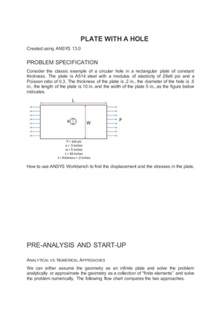
Consider the classic example of a circular hole in a rectangular plate of constant
thickness. The plate is A514 steel with a modulus of elasticity of 29e6 psi and a
Poisson ratio of 0.3. The thickness of the plate is .2 in., the diameter of the hole is .5
in., the length of the plate is 10 in. and the width of the plate 5 in., as the figure below
indicates.
How to use ANSYS Workbench to find the displacement and the stresses in the plate.
PRE-ANALYSIS AND START-UP
ANALYTICAL VS. NUMERICAL APPROACHES
We can either assume the geometry as an infinite plate and solve the problem
analytically or approximate the geometry as a collection of "finite elements” and solve
the problem numerically. The following flow chart compares the two approaches.

Let's first review the analytical results for the infinite plate. We'll then use these results
to check the numerical solution from ANSYS.
ANALYTICAL RESULTS
DISPLACEMENT
Let's estimate the expected displacement of the right edge relative to the center of the
hole. We can get a reasonable estimate by neglecting the hole and approximating the
entire plate as being in uniaxial tension. Dividing the applied tensile stress by the
Young's modulus gives the uniform strain in the x direction.
Multiplying this by the half-width (5 in) gives the expected displacement of the right
edge as ~ 0.1724 in. We'll check this against ANSYS.
SIGMA-R
Let's consider the expected trends for Sigma-r, the radial stress, in the vicinity of the
hole and far from the hole. The analytical solution for Sigma-r in an infinite plate is:

where a is the hole radius and Sigma-o is the applied uniform stress (denoted P in the
problem specification). At the hole (r=a), this reduces to
This result can be understood by looking at a vanishingly small element at the hole as
shown schematically below.
We see that Sigma-r at the hole is the normal stress at the hole. Since the hole is a
free surface, this has to be zero.
For r>>a,
Far from the hole, Sigma-r is a function of theta only. At theta = 0, Sigma-r ~ Sigma-
o. This makes sense since r is aligned with x when theta = 0. At theta = 90 deg., Sigma-
r ~ 0 which also makes sense since r is now aligned with y. We'll check these trends
in the ANSYS results.
SIGMA-THETA
Let's next consider the expected trends for Sigma-theta, the circumferential stress, in
the vicinity of the hole and far from the hole. The analytical solution for Sigma-theta in
an infinite plate is:

At r = a, this reduces to
At theta = 90 deg., Sigma-theta = 3*Sigma-o for an infinite plate. This leads to a stress
concentration factor of 3 for an infinite plate.
For r>>a,
At theta = 0 and theta = 90 deg., we get
Far from the hole, Sigma-theta is a function of theta only but its variation is the opposite
of Sigma-r (which is not surprising since r and theta are orthogonal coordinates; when
r is aligned with x, theta is aligned with y and vice-versa). As one goes around the hole
from theta = 0 to theta = 90 deg., Sigma-theta increases from 0 to Sigma-o. More
trends to check in the ANSYS results!
TAU-R-THETA
The analytical solution for the shear stress Tau-r-theta in an infinite plate is:
At r=a,
By looking at a vanishingly small element at the hole, we see that Tau-r-theta is the
shear stress on a stress surface, so it has to be zero.

For r>>a,
We can deduce that, far from the hole, Tau-r-theta = 0 both at theta = 0 and theta =
90 deg. Even more trends to check in ANSYS!
SIGMA-X
First, let's begin by finding the average stress, the nominal area stress, and the
maximum stress with a concentration factor.
The concentration factor for an infinite plate with a hole is K = 3. The maximum stress
for an infinite plate with a hole is
Although there is no analytical solution for a finite plate with a hole, there is empirical
data available to find a concentration factor. Using a Concentration Factor Chart
(Cornell 3250 Students: See Figure 4.22 on page 158 in DeformableBodies and Their

Material Behaviour), we find that d/w = 1 and thus K ~ 2:73 Now we can find the
maximum stress using the nominal stress and the concentration factor
OPEN ANSYS WORKBENCH
Now that we have the pre-calculations, we are ready to do a simulation in ANSYS
Workbench! Open ANSYS Workbench by going to Start > ANSYS > Workbench. This
will open the start-up screen as seen below
To begin, we need to tell ANSYS what kind of simulation we are doing. If you look to
the left of the start-up window, you will see the Toolbox Window. Take a look through
the different selections. The plate with a hole is a static structural simulation. Load the
static structural tool box by dragging and dropping it into the Project Schematic.
Name the Project "Plate with a Hole" by double clicking the text Static
Structural and typing in Plate with a Hole.

MATERIAL SELECTION
Now we need to specify what type of material we are working with. Double
click Engineering Data and it will take you to the Engineering Data Menus.
If you look under the Outline of Schematic A2: Engineering Data Window, you will see
that the default material is Structural Steel. The Problem Specification specifies the
material's Modulus of Elasticity and Poisson's ratio. To add a new material, click in an
empty box labelled Click here to add a new material and give it a name. We will call
our material Cornellium.
On the left-hand side of the screen in the Toolbox window, expand Linear Elastic and
double click Isotropic Elasticity to specify the Elastic Modulus and Poisson's Ratio.

In the Properties of Outline Row 4: Cornellium window, Set the Elastic Modulus units
to psi, set the magnitude as 29e6, and set the Poisson's Ratio to .3.
Close the materials window by selecting Return to Project.
Now that the material has been specified, we are ready to make the geometry in
ANSYS.
GEOMETRY
For users of ANSYS 15.0, please check this link for procedures for turning on the Auto
Constraint feature before creating sketches in DesignModeler.
ANALYSIS TYPE
First, right click and click Properties to bring up the geometry
properties menu. The default analysis type of ANSYS is 3D, but we are doing a 2-
dimensional problem. Change the Analysis Type from 3D to 2D.

Next double click . This will bring up the Design Modeler. It
will prompt you to pick the standard units. Since all the units in the problem
specification were given in English units, we want to choose inch. When
the Inch radio button is selected, press OK
DRAW THE GEOMETRY
To begin sketching, we need to look at a plane to sketch on. Click on the Z-axis of the
compass in the bottom right hand corner of the screen to look at the x-y plane.

Now, look to the sketching toolboxes window and click the sketching tab; this will bring
up the sketching menu.
Before we sketch the geometry, let's note something about the problem specification.
The geometry itself has two planes of symmetry: it is symmetric about the x-plane and
y-plane. This means we can model 1/4 of the geometry and use symmetry constraints
to represent the full geometry in ANSYS. If me model a quarter of the geometry, we
can make the problem less complex and save some computational time.
Okay! Let's start sketching. First, click in the sketching tool bar. This tool
defines a rectangle by two points. Place the first point at the origin (Watch for the P-
symbol which shows you are placing the point at the origin point), and the other point
somewhere in the first quadrant.

Now, click . This tool allows to define a circle by clicking once to define its
centre point, then click a distance away from the centre point to define a radius. Define
the circle so its centre point is at the origin, define the radius by clicking somewhere
inside the rectangle.
We almost have a geometry, but we first need to get rid of the superfluous lines. In the
sketching toolboxes window, click Modify > Trim.
Now, trim the segments that are 1. outside of the 1st quadrant, and 2. between the
circle and the origin. You should end up with something similar to the following figure.

DIMENSIONS
Now, we must dimension the drawing to the problem specification. (Remember! We
are only drawing 1/4 of the geometry, so we need to take this into account when
dimensioning the figure in ANSYS). In the sketching toolboxes window,
click Dimensions > General
This tool will allow you to define dimensions that you can specify. We need to specify
the rectangle's length and width, and the circle's radius. Use the tool to define the
height of the rectangle (the right edge of the geometry), the length of the rectangle (the
top edge of the rectangle), and the radius of the circle. You should end up with the
following window.

To specify the dimensions, look to the Details View Window.
Change the H (for horizontal) dimension to 5 inches, the V (for vertical) dimension to
2.5 inches, and the R (for radius) dimension to .25 inches. Now we have the geometry
specified in the problem statement sketched in ANSYS.

CREATE A SURFACE FROM THE SKETCH
Next, we need to tell ANSYS what type of geometry we are modelling. For this
problem, we will create a surface and give it a thickness. In the menu bar,
select Concept > Surfaces from Sketches. To select the sketch, look to the outline
window, and expand XY plane > Sketch 1 .
In the details window pane, select Base Objects > Apply . Now, we need to specify
a thickness. Specify the thickness as .1 inches, as from the problem statement. Now
in the menu toolbar, click This should generate the geometry.
Close the Deign Modeler (don't worry, the geometry will be saved in the project
automatically). Now we are ready to mesh the geometry.

MESH
FACE SIZING
Now, double click Model in the project outline to bring up the Mechanical window.
Go to Units > U.S. Customary (in. lbm, lbf, F, s, V, A) to make sure the proper units
are selected.

To begin the Mesh process, click Mesh in the outline window. This will bring up the
Mesh Menu bar in the Menu bar.
We want to control the size of the elements in the mesh for this problem; to accomplish
this, click Mesh Control > Sizing. We now need to pick the geometry we are going to
mesh. Make sure the Face Selection Filter is selected then click the face of the
geometry to select it. In the Details window click Geometry > Apply. Now, we can set
some of the details of our mesh. Select Element Size > Default, this will allow you to
change the size of the element. Choose the size of the elements to be .05 in.
Turn off the Advanced Size Function in the details window of "Mesh". If we leave
the Advanced Size Function on, ANSYS will override the face sizing we applied.

EDGE REFINEMENT
Now, we want to refine the mesh by the hole, where we expect a stress concentration.
Go to Mesh Control > Refinement. This will open the Refinement menu if the details
view window. To select the hole as the geometry for refinement, make sure the edge
select tool is selected from the menu toolbar. Now, select the
hole's edge then click Geometry > Apply.

In the details window, change the Refinement parameter from 1 to 3, this will give us
the finest mesh at the hole which will improve accuracy of the simulation.
Now that we have our mesh setup, click Mesh > Generate Mesh. This will create the
mesh to our specifications. Click to display it. It should look something
like this:
Now that the mesh has been created, we are ready to specify the boundary conditions
of the problem.
PHYSICS SETUP
SPECIFY MATERIAL
First, we will tell ANSYS which material we are using for the simulation.
Expand Geometry, and click Surface Body in the Outline window. In
the Details window, select Material > Assignment > Cornellium. The material has
now been specified.

Click here to enlarge
SYMMETRY CONDITIONS
First, let's start by declaring the symmetry conditions in the problem. Right click Model
> Insert > Symmetry.
This will create a symmetry folder in the outline tree Now, right
click Symmetry > Insert > Symmetry Region. Make sure the Edge Select Tool is
highlighted and select the left edge above the hole.

Now look to the Details View window and select Geometry > Apply. This should
create a red line with a tag on the model. Ensure that under Symmetry Normal the x-
axis is selected. Repeat this process to create a symmetry region for the bottom edge
to the right of the hole, but this time making sure that the Symmetry
Normal parameter is the y-axis.
FORCES
Now, we can specify the forces on the body. Click Static Structural in the outline tree.
This will bring up the Physics Sub-Menu bar in the Menu Bar.

Click Loads > Pressure to specify a traction. Select the right edge of the geometry
and apply it in the details view window. The pressure's magnitude from the problem
specification is -1e6 psi (pressure in ANSYS defaults to compression, and we need
tension, hence the negative sign). Now that the forces have been set, we need to set
up the solution before we solve.
NUMERICAL SOLUTION
Now we are ready to choose what kind of results we would like to see.
DEFORMATION
To add deformation to the solution, first click Solution to add the solution sub menu
to menu bar
Now in the solution sub menu click Deformation > Total to add the total deformation
to the solution. It should appear in the outline tree.
NORMAL STRESSES
SIGMA_XX
To add the normal stress in the x-direction, in the solution sub menu go to Stress >
Normal. In the details view window ensure that the Orientation is set to X Axis. Let's
rename the stress to Stress_xx by right clicking the stress, and going to rename.
SIGMA_R
To add the polar stresses, we need to first define a polar coordinate system. In the
outline tree, right click Coordinate System > Insert > Coordinate System.
This will create a new Cartesian Coordinate System. To make the new coordinate
system a polar one, look to the details view and change the Type Parameter from
Cartesian to Cylindrical. To define the origin, change the Define By parameter from
Geometry to Global Coordinate System. Put the origin coincident with the global
coordinate systems origin (x = 0, y = 0). Now that the polar coordinates have been

created, lets rename the coordinate system to make it more distinguishable. Right click
on the coordinate system you just created, and go to Rename. For simplicity sake,
let's just name it Polar Coordinates.
Click here to enlarge image
Now, we can define the radial stress using the new coordinate system. Click Solution
> Stress > Normal. This will create "Normal Stress 2” and list its parameters in the
details view. We want to change the coordinate system to the polar one we just
created; so, in the details view window, change the Coordinate System parameter
from "Global Coordinate System" to "Polar Coordinates". Ensure that the orientation
is set to the x-axis, as defined by our polar coordinate system. Now the stress is ready.
Let's rename it to Sigma_r and keep going.
SIGMA_THETA
Now let's add the theta stress. This is too a normal stress, so create a new normal
stress as you did for Sigma_xx and Sigma_r. Now, change the coordinate system to
Polar Coordinates, as you did for Sigma-r. Next, change the Orientation to the Y axis.
The Y axis should be in the theta direction by default. Rename the stress
to Sigma_theta.

TAU_R-THETA
Finally, let's add the shear stress in the r-theta direction. To do this, we go to Solution
> Stress > Shear. You'll notice that now, in the details view window, the stress needs
two directions to define it. In order to solve for the r-theta shear, we need to change
the Coordinate Systemparameter from the Global Coordinate System to Polar
Coordinates. Also, ensure that the Orientation is in the XY direction (in polar, this will
be r_theta by the coordinate system we created). Rename the stress to Tau_r-theta.
This is what your outline tree should look like at this point:

SOLVE!
To solve for the stresses and deformation, we now hit the solve button.
Keep going! Almost done!
NUMERICAL RESULTS
DISPLACEMENT
Okay! Now let's look at the numerical solution to the boundary value problem as
calculated by ANSYS. Let's start by examining how the plate deformed under the load.
Before you start, make sure the software is working in the same units you are by
looking to the menu bar and selecting Units > US Customary (in, lbm, lbf, F, s, V,
A). Also, select the pan tool by clicking the pan button from the top bar. This will
allow you to zoom by scrolling the mouse wheel, and move the image by left-clicking
and dragging.
Now, look at the Outline window, and select Solution > Total Deformation. First, we
will look at just the deformation of the plate, without contours. To do this, select the
Contours button, , and select Solid Fill.

There are a few things we can determine from this picture. Let's use our intuition and
the work we did in the pre-analysis to compare to the result ANSYS gives us. First,
let's look at the bottom and left edges of the plate. We can see that the deformation
on these edges is parallel to the sides, which agrees with the symmetry boundary
condition. The top edge of the plate has deformed downwards, which is due to the
effects of Poisson's ratio. The right edge has moved to the right, which is consistent
with the expected behavior, due to the plate being in tension. So we can deduce the
following boundary conditions from looking at the deformation.
Animate the deformation by pressing Play in the Animation tool bar along the bottom
of the screen. This linearly interpolates between the initial and final deformed state.
To get back the color contours of deformation values, select the Contours button and
choose Contour Bands. The colored section refers to the magnitude of the
deformation (in inches) while the black outline is the undeformed geometry
superimposed over the deformed model. The more red a section is, the more it has
deformed while the more blue a section is, the less it has deformed. Notice that far
from the hole, the deformation is linearly varying, similar to a bar in tension. Now let's
look at the value of the largest deformation. Looking at the top of the color bar, we see
that the largest deformation is 0.176 inches. From our pre-analysis, we estimated that

the deformation was ~ 0.17 inches - a 2% difference. This is one check on our ANSYS
result.
SAVE IMAGE TO A FILE
You can save the image to a file using the Image to File option shown below.
Sometimes, you get an error saying "The display settings are Windows Aero and
image capture might not work." In that case, you can use the Windows 7 snipping tool
which can be accessed from the Start > Programs menu as shown below.
Draw a rectangle around the screen area that you want to capture and save to an
image file.
SIGMA-R
Now let's look at the radial stresses in the plate. Look to the outline window and
click Solution > Sigma-r. This will display the radial stresses.
Does this match what we expect? First, let's examine the hole at r = a. From our pre-
calculations, we found that the stress at the hole in the radial direction should be 0.
Zooming in with the middle mouse wheel and using our probe tool, we find that the
stress in this area ranges from -450 to 450 psi. Although the simulation does not
approach exactly zero, keep in mind that 450 psi is less than 1% of the average stress,
so it can be thought of as approximately zero. Also, we expect this value to get closer
to zero as we refine the mesh.
In order to zoom out and view the whole solution, select the zoom to fit button from
the toolbar.

Now, let's first look at the case when r >> a. As we found in the pre-calculations, when
r >> a, the radial stress is a function of the angle theta only. This matches the behavior
seen in the simulation. From our Pre-Calculations, we also found that .
Using the probe tool, we find that indeed at this location, the stress is equal to 1e6 psi,
which is the value we calculated in our Pre-Analysis. Also from our Pre-Analysis, we
found that when .
Checking the simulation with our trusty probe tool, we find that the ANSYS simulation
matches up quite nicely with our calculation.
SIGMA-THETA
Now, let's compare the simulation to our pre-calculations for the theta stress. Look to
the Outline window, then click Solution > Sigma-theta
First, let's compare the case when r = a. From the pre-analysis, we found that the
stress at the hole acts as a function of theta. Specifically:
From this equation, we find that at zero degrees, we expect the stress to be -1e6 psi
at zero degrees and at 90 degrees, we expect the stress to be 3e6 psi. Zoom in close
to the hole to view the stresses there. From the simulation we find that the stress at 0
degrees is -1.0285e6 psi (a 3% deviation), and the stress at 90 degrees is 3.0323e6
psi (a 1 % deviation). The deviations are due to the infinite plate assumption in the
theory.
Now, let's look at the case when r >> a. From our pre-calculations, we found that the
theta stress is a function of theta only. This behaviour is represented in the simulation.
Also, for r >> a and the stress is equal to .
Using the probe tool and hovering over this area, we see that the stress is indeed
equal to Sigma-o. However, looking at the area when , we find that the stress
from the simulation is between 1000 psi and 2000 psi. Although this seems large
compared to zero, one must keep in mind that the stress at this location is 1% of the
average stress. We expect that the stress here will get closer to zero on refining the
mesh since the numerical error becomes smaller.

TAU-R-THETA
Now let's look at how the simulation match our predictions for the shear stress. Look
to the Outline window, then click Solution > Tau-r-theta
In our pre-analysis, we determined that at r = a the shear stress should be 0 psi. Using
our probe tool, we find that the stress ranges between -5 and -500 psi at the hole.
Because 500 psi is .05% of the average stress, we can say this result does represent
what we expect to happen very well.
In our pre-calculations, we determined that far from the hole the shear stress should
be a function of theta only. This can be shown by using the probe tool a hovering over
a radial line from the hole. The colors (representing higher and lower stresses) only
change only as the angle changes, but not as the move away from the hole. We also
found that far from the hole at the stress is zero
Using the probe tool, we can see that this is indeed the case for the simulation as well.
SIGMA-X
Now let’s examine the stress in the x-direction. Look to the Outline window, then
click Solution > Sigma-x
From this, you can see that most of the plate is in constant stress, and there is a stress
concentration around the hole. The more red areas correspond to a high, tensile
(positive) stress and the bluer areas correspond to areas of compressive (negative)
stress. Let's use the probe tool to compare the ANSYS simulation to what we expected
from calculation. In the menu bar, click the Probe button; this will display the Sigma-x
values at the cursor location as you hover over the
plate.
Start by hovering over the area far from the hole. The stress is about 1e6 psi, which is
the value we would expect for a plate in uniaxial tension. If you click the max tag

(located adjacent to the probe tool in the menu bar), it will locate and display the
maximum stress, which is shown as 3.0335e6 psi. This is about a 0.0055% difference
from the calculation we did in the Pre-Analysis, which is a negligible difference.
SIGMA-X ALONG AN EDGE
The stress along the left edge of the model can be found very easily. Remember, this
is a quarter model, hence the left edge of the model is actually the center line of the
full plate. In the Outline tree, insert Construction Geometry as shown in the following
figure:
Right click on construction geometry and insert a path and rename it "left edge".

Enter the following start and end coordinates:
You should see a gray path displayed on the left edge of the model.
Add a normal stress object under Solution in the tree: Stress > Normal. Change the
scoping method to Path and select left edge for Path.
Click on Solve to generate the result. ANSYS Mechanical will plot the stress along the
left edge and the data is tabulated.

You can export the tabular data in Excel or text format by right-clicking on it.
Verification & Validation
Now that we have our results, it is important that we check to see that our
computational simulation is accurate. One possible way of accomplishing this task is
comparing to the pre-calculations, as we did in the results section. Another way to
check our results is by refining the mesh further. The smaller the elements in the mesh,
the more accurate our simulation will be, but the simulation will take longer. To refine
the mesh, look to the outline tree and click Mesh > Face Sizing Change the element
sizing to 0.025 in (half the size of the mesh we originally tried). The new mesh looks
like this . It has twice as many elements as the original.
Now hit solve. Compare the values for your stresses with those we found for the
original mesh. Are the very different? Or do they seem to approach a limit? If the latter,
the mesh is refined enough and if you modeled the problem correctly, you are done!
Below are the values from our original mesh, followed by the values for our refined
mesh.
Maximum Sigma_xx Maximum Deformation
Theory Values 3.0033 x 10^6 psi 0.1724
Original Mesh 3.0336 x 10^6 psi 0.1761
Refined Mesh 3.0360 x 10^6 psi 0.1759
As one can see from the table above the results do not change greatly as the mesh is
refined. This means we don't need to refine the mesh further.
We're Done!

TENSILE BAR (RESULTS-INTERPRETATION)
A steel bar is mounted in a rigid wall and axially loaded at the end by a force P = 2 kN
as shown in the figure below. The bar dimensions are indicated in the figure. The bar
is so thin that there is no significant stress variation through the thickness. Neglect
gravity.
The material properties are:
 Young's modulus E = 200 GPa
 Poisson ratio = 0.3
In this exercise, you are presented with the numerical solution to the above problem
obtained from finite-element analysis (FEA) using ANSYS software. Compare FEA
results for the stress distribution presented to you with the corresponding analytical
solution. Justify agreements and discrepancies between the two approaches (FEA vs.
Analytical).
PRE-ANALYSIS AND START-UP
In the Pre-Analysis step, we'll review the following:
 Mathematical model: We'll look at the governing equations + boundary conditions
and the assumptions contained within the mathematical model.
 Hand-calculations of expected results: We'll use an analytical solution of the
mathematical model to predict the expected stress field from ANSYS. We'll pay close
attention to additional assumptions that have to be made in order to obtain an
analytical solution.

 Numerical solution procedure in ANSYS: We'll briefly overview the solution
strategy used by ANSYS and contrast it to the hand calculation approach.
MATHEMATICAL MODEL
We'll first list the assumptions in the mathematical model. Then, we'll review the
governing equations and boundary conditions that form the mathematical model. Note
that this type of a mathematical model where you have a set of differential equations
together with a set of additional restraints at the boundaries is called a Boundary Value
Problem (BVP). A lot of practical problems that are solved using ANSYS and other
FEA software are BVP's. You should have encountered simple BVP's in your math
courses, problems of the kind that involve solving a differential equation with a set of
boundary conditions (I was never good at these math problems and it showed in my
math grades to the displeasure of my parents .... fortunately that is now a distant
memory!). You can think of the BVP considered in this tutorial as a souped-up version
of simpler BVP's you have encountered in math courses (and either liked or hated!).
ASSUMPTIONS
We'll assume that:
1. Plane stress conditions apply since the bar is thin, thus we don't expect significant
variation of stresses in the z direction:
2. Gravity effects can be neglected i.e. no body forces.
GOVERNING EQUATIONS
Since we are assuming plane stress conditions, we can use the 2D version of the
equilibrium equations. When the deformed structure reaches equilibrium, the 2D
stress components should satisfy the 2D equilibrium equations with zero body forces:
BOUNDARY CONDITIONS
We solve these equations in a rectangular domain and impose the appropriate
boundary conditions. At every point on the boundary, either the displacement or the
traction must be prescribed.

The bottom and top edges are free. If a boundary location is not constrained and can
move freely, it can expand and contract without incurring stress. Thus, traction on the
free edges is zero and we get
The left end is fixed. So both components of displacement are zero at this end:
The boundary condition is a little bit more complicated at the right end. Here, the
traction is specified at the mid-point where the point load is applied. The applied
traction at all other points on the right boundary is zero. For brevity, we won't write out
the corresponding equations at the right boundary. We'll simplify this boundary
condition in our hand calculations below (to make the problem tractable) but the
ANSYS solution provided uses the full set of boundary conditions. Another
complication is that since we have a point load, the specified traction at the mid-point
of the right end is infinite. We'll later discuss the effect of this in the ANSYS solution.
Do keep in mind that there are no point loads in practice, it's just an idealization that
can lead to weird behaviour that we need to be aware of.
HAND CALCULATIONS
Now that we have reviewed the mathematical model for our problem, let's hold off
diving into ANSYS just yet and first make some hand calculations of expected results.
We'll use these hand calculations to check ANSYS results (like an expert engineer
would!). In order to make the problem solvable by hand, we need to make additional
assumptions. The ANSYS solution does not make these additional assumptions.
ADDITIONAL ASSUMPTIONS IN HAND CALCULATIONS
1. We'll simplify the right boundary condition. Instead of a point load, we'll assume that
the load is distributed over the entire right boundary. So, the traction condition at the
right boundary becomes

Here, t is the thickness.
The following schematic shows the process of simplifying the right boundary
condition in the hand calculation.
2. Away from the left and right ends, we expect a uni-axial state of stress with zero shear
(OK, this is a bit of a leap of the imagination but it's plausible). So, we'll assume that
everywhere
We don't expect this to hold near the left boundary or in the vicinity of the point load,
so our hand calculations won't be valid there.
ANALYTICAL SOLUTION
With these additional assumptions in hand, we can easily solve the BVP and we get
the following analytical solution:
This is the well-known (P/A) result but we have arrived at it somewhat carefully,
accounting for the additional assumptions we made in the process. We'll need to keep
these additional assumptions in mind when comparing the hand calculations with the
ANSYS solution. For the values given in the problem statement, we have

The corresponding strain in the x-direction can be calculated from Hooke' law:
The strain is tiny since the material is very stiff with a Young's modulus of 200 GPa.
The displacement at the right end can be estimated by integrating the constant x-
strain:
The above hand calculations give us expected values of stress, strain and
displacement which we'll compare with the ANSYS results.
NUMERICAL SOLUTION PROCEDURE IN ANSYS
The type of numerical solution procedure used by ANSYS is called finite-element
analysis (FEA) or finite-element method (FEM). In FEA, we divide or "discretize" the
domain into small rectangles or "elements" (hence the name finite element analysis).
ANSYS obtains the numerical solution to the BVP in the discrete domain. ANSYS
directly solves for the u and v displacements at selected points called "nodes".
Everything else such as the stress variation is derived from these nodal displacements
through interpolation. The nodes in our case are the corners of the elements as shown
below. As you can imagine, the numerical solution should get better as you increase
the number of elements.
The following figure summarizes the contrasts between the hand calculations and
ANSYS's approach. One important point to keep in mind is that both start with the
same mathematical model but use different assumptions and approximations to solve
it. Also, in FEA, one always computes the displacement first and from that derives the
stress. Contrast that to the hand calculations where we calculated the stress first and
from that derived the displacement. The latter process works only for a few simple
problems.

This brings us to the end of the Pre-Analysis section.
START-UP: LOAD SOLUTION INTO ANSYS
As mentioned before, we are providing the ANSYS solution so that you can focus on
comparing the hand calculations with the ANSYS results (which is the goal of this
exercise). Without further ado, let's download the ANSYS solution and load it into
ANSYS.
1. Download "Tensile Bar Demo.zip" by clicking here
Unzip the file at a convenient location. You will see a folder called Tensile Bar
Demo with the following contents:
 Tensile Bar Demo_files (this is a folder)
 Tensile Bar Demo.wbpj
Please make sure both these objects are in the unzipped folder, otherwise the solution
will not load into ANSYS properly. (Note: The solution provided was created using
ANSYS workbench 13.0 release, there may be compatibility issues when attempting
to open with older versions).
2. Double click "Tensile Bar Demo.wbpj" - This should automatically open ANSYS
Workbench (you have to twiddle your thumbs a bit before it opens up). You will then
be presented with the ANSYS solution in the project page.

A tick mark against each step indicates that that step has been completed.
3. To look at the results, double click on Results - This should bring up a new window
(again you have to twiddle your thumbs a bit before it opens up).
4. On the left-hand side there should be an Outline toolbar. Look for Solution (A6).
We'll investigate the items listed under Solution (A6) in the next step of this tutorial.
NUMERICAL RESULTS
Before we explore the ANSYS results, let's take a peek at the mesh.
MESH
Click on Mesh (above Solution) in the tree outline. This shows the mesh used to
generate the ANSYS solution. The domain is a rectangle. This domain is discretized
into a number of small "elements". Recall that ANSYS solves the BVP and calculates
the displacements at the nodes. A finer mesh is used near the left and right ends where
we expect greater stress concentration. We have checked that the solution
presented to you is reasonably independent of the mesh.

UNITS
Set the units for the results display by selecting Units > Metric (mm, kg, N, s, mV,
mA) . The displacements will be reported in mm and the stresses in N/mm2 which is
equivalent to MPa.
DISPLACEMENT
To view the deformed structure, click on Solution > Displacement in the tree outline.
The black rectangle shows the undeformed structure. The deformed structure is
colored by the magnitude of the displacement. The displayed displacement distribution
is calculated by interpolating the nodal displacements. Red areas have deformed more
and blue areas less. You can see that the left end has not moved as specified in the
problem statement. This means this boundary condition has been applied correctly.
The displacement increases from left to right as we intuitively expect. There is also not
much variation in the y-direction. So, we can conclude that the model has been
constrained properly.
Note the extremely high deformation near the point load. This extremum is unrealistic
and should be ignored (there are no point loads in reality).
To view the Poisson effect (shrinking in the y direction), zoom into the top-rightright
corner by drawing a rectangle around the region with the right mouse button.

You can do this multiple time to zoom in more. You do indeed see the shrinking in the
y-direction as expected but it is small for this model.
You can restore the front view of the entire model by right-clicking in the background
and choosing View > Front .
Note that you can zoom in and out using the middle mouse wheel. You can translate
the model by clicking on the Pan button and dragging the model with the left mouse
button. There are also a bunch of zoom options next to the Pan button.

SIGMA_X
investigating sigma_x:
1. Click on probe and hover over the bar. Using the probe may tell you the stress
associated with a specific point on the bar.
2. To view the less noticeable stress contours, click on the scale to edit. In this video,
the orange (2nd highest value) was changed to 250 and the blue (2nd lowest value)
was changed to 50. The contour map changed to display the subtle difference in
sigma_x.
In the video, we saw that ANSYS's values for sigma_x matches with:
 The analytical solution in the interior (away from the left and right boundaries)
 Traction boundary condition for sigma_x at the right boundary
Note that sigma_x at the location of the point load is infinite. So as the mesh is
refined further, sigma_x at the point load will get larger and larger without bound.
SIGMA_Y
Next, let's take a look at sigma_y. Click on Solution > sigma_y in the tree outline.
Again, probe values in the middle as well as at the ends. Check that:
 The value away from the boundaries is close to zero as expected from the analytical
solution. It is not exactly zero because of round-off errors.
 The value at the top and bottom boundaries are close to zero. This agrees with the
boundary condition at these boundaries since the traction has to be zero at these
free boundaries. In other words, the normal component of the traction acting on
these surfaces is sigma_y and that has to be zero since the traction on these free
surfaces is zero.
 There is significant deviation from the analytical solution at both ends. The analytical
solution breaks down at these ends because of the additional assumptions that we
made. Note that there are areas where sigma_y is negative i.e. compressive.

TAU_XY
We expect tau_xy to be zero away from the ends. Near the ends, since sigma_x and
sigma_y are non-zero, we expect
Plot tau_xy, look at the range of values and use Probe to check actual values. Are the
above statements valid?
EQUIVALENT STRESS (VON MISES):
The Equivalent or Von Mises stress is used to predict yielding of the material. We can
see that the analytical solution under-predicts the maximum equivalent stress. Thus,
one would need to use a large factor of safety if using the analytical result while
designing such a structure. One would use a factor of safety with the FEA result also,
but it does not have to be as large.
VERIFICATION AND VALIDATION
One can think of Verification and Validation as a formal process for checking results.
Each of these terms has a specific meaning which we won't get into here. We have
already done some checks on the ANSYS results by comparing them to the hand
calculations and checking that the ANSYS solution agrees with the appropriate traction
or displacement boundary condition at each boundary. Let's next check ANSYS's
displacement value at the right boundary with the value in our hand calculations.
CHECK DISPLACEMENT VALUE AT THE RIGHT BOUNDARY
 Bring up the Displacement result again by clicking on that object in the tree.
 I prefer to turn off the deformation in the view as per snapshot below.
 Zoom into the right end using the right mouse button.

 Click Probe and check the displacement values away from the point load.
I get a value around 0.045 mm at the right end away from the point load. This is about
a 10% deviation from the hand calculation result of 0.05 mm we obtained in our Pre-
Analysis.This is a reasonable agreement considering that the hand calculation ignores
the high stress areas at the left and right ends. But these high stress areas (both tensile
and compressive) affect relatively small areas of the model and so don't contribute a
lot to the overall displacement.
SUMMARY OF OUR RESULT CHECKS
1. The stress components agree well with hand calculations away from the right and
left ends.
2. The displacement at the right end (away from the point force) is within about 10%
from the hand calculation value.
3. The ANSYS solution agrees with the boundary conditions on traction as well as
displacement.
Thus, we can be reasonably confident that the ANSYS model has been set-up
correctly. We have however not checked that we have resolved the high stresses at
the left and right ends correctly. So we cannot say anything about when the part would
fail. Further mesh refinement may be needed. We also should get rid of the stress
singularity at the point load (by distributing it over a region) and at the left corners (by
filleting these corners).

CANTILEVER BEAM MODAL ANALYSIS
Created using ANSYS 13.0
Consider an aluminum beam that is clamped at one end, with the following
dimensions.
Length 4 m
Width 0.346 m
Height 0.346 m
The aluminum used for the beam has the following material properties.
Density 2,700 kg/m^3
Youngs Modulus 70x10^9 Pa
Poisson Ratio 0.35
Using ANSYS Workbench find the first six natural frequencies of the beam and the
mode shapes.
PRE-ANALYSIS & START-UP
PRE-ANALYSIS
The following equations give the frequencies of the modes and the mode shapes and
are derived from Euler-Bernoulli Beam Theory.

START ANSYS WORKBENCH & LOAD FILES
In this section we will launch ANSYS Workbench and then load the project file,
"cantilever.wbpj" that was created in the "Cantilever Beam" tutorial.
Start > All Programs > ANSYS 12.1 > Workbench
File > Open
Then choose the "cantilever.wbpj" file that you created in the "Cantilever Beam"
tutorial.
MANAGEMENT OF SCREEN REAL ESTATE
This tutorial is specially configured, so the user can have both the tutorial and ANSYS
open at the same time as shown below. It will be beneficial to have both ANSYS and
your internet browser displayed on your monitor simultaneously. Your internet browser
should consume approximately one third of the screen width while ANSYS should take
the other two thirds as shown below.

Click Here for Higher Resolution
If the monitor you are using is insufficient in size, you can press the Alt and Tab keys
simultaneously to toggle between ANSYS and your internet browser.
MODAL (ANSYS) PROJECT SELECTION
Left, click on Modal ANSYS, , and drag it to the right of the "Cantilever"
project. You should then see a red box to the right of the "Cantilever" project that says
"Create standalone system" as shown below.
Higher Resolution Image
Now, release the left mouse button. Your Project Schematic window should now look
comparable to the image below.

RENAME MODAL (ANSYS)
Double click on Modal (ANSYS) and rename it to "Cantilever Modal".
ENGINEERING DATA
In this section we will input the properties of aluminum (as defined in the the Problem
Specification) in to ANSYS. First, double click Engineering Data,
, in the "Cantilever Modal" Project. Next, click where it says "Click
here to add a new material" as shown in the image below.

Next, enter "Aluminum" and press enter. You should now have Aluminum listed as
one of the materials in table called "Outline of Schematic B2: Engineering Data", as
shown below.
Then, (expand) Linear Elastic, as shown below.
Now, (Double Click) Isotropic Elasticity. Then set Young's Modulus to 70e9 Pa
and set Poisson's Ratio to 0.35 , as shown below.

Next, (expand) Physical Properties, as shown below.
Now, (Double Click) Density. Then, set Density to 2,700 kg / m^3 , as shown below.
Now, the material properties for Aluminum have been specified. Lastly, (Click) Return
To Project, .

SAVE
Save your project now and periodically, as you work. ANSYS does not have an auto-
save feature.
GEOMETRY
For users of ANSYS 15.0, please check this link for procedures for turning on the Auto
Constraint feature before creating sketches in DesignModeler.
ATTACH GEOMETRY FROM CANTILEVER TO CANTILEVER MODAL
The geometry for the "Cantilever Beam Modal Analysis" tutorial is the same as the
geometry for the "Cantilever Beam" tutorial. Instead of recreating the geometry, we
will simple attach the geometry from the Static Structural Analysis System (Cantilever)
to the Modal Analysis System (Cantilever Modal). In order to attach the geometry, (left
click) Geometry in the "Cantilever" project and drag it to Geometry in the "Cantilever
Modal" project, as shown below.
Then release the left mouse button. You should now see that the geometries are
shared as shown in the following image.
MESH
LAUNCH MECHANICAL
(double click) Model, , in the "Cantilever Modal" project.

GENERATE DEFAULT MESH
First, (click) Mesh in the tree outline. Next, (click) Mesh > Generate Mesh as shown
below.
SIZE MESH
In this section we will size the mesh, such that it has ten uniform elements. In order to
size the mesh, first expand Sizing located within the
Details of "Mesh" table. Next, set Element Size to 0.40 m, as shown below.
Now, (click) Mesh > Generate Mesh in order to generate the new mesh. You should
obtain the mesh, that is shown in the following image.

Note that in this simulation we are working with beam elements, which are simply line
segments. As a visualization tool ANSYS displays a beam with width and height. In
order to display the actual mesh (click) View > (deselect) Thick Shells and Beams.
You will then see the mesh displayed in its native form.
PHYSICS SETUP
MATERIAL ASSIGNMENT
At this point, we will tell ANSYS to assign the Aluminum material properties that we
specified earlier to the geometry. First, (expand) Geometry then (click) Line Body,
as shown below.
Then, (expand) Material in the "Details of Line Body" table and set Assignment to
Aluminum, as shown below.

At this point your "Details of Line Body" table, should look comparable to the following
image.
FIXED SUPPORT
First, (right click) Modal > Insert > Fixed Support, as shown below.

Next, click the vertex selection filter button, . Then, click on the left end of the
beam and apply it as the Geometry in the "Details of Fixed Support" table.
CONSTRAIN BEAM TO XY PLANE
In this section the beam's motion will be constricted to the xy plane.
First, (right click) Modal > Insert > Displacement, as shown below.
Next, click the edge selection filter button, . Then, click on the geometry and
apply it as the Geometry in the "Details of Displacement" table. Lastly, set Z
Component to 0, as shown below.

NUMERICAL SOLUTION
SPECIFY RESULTS (DEFORMATION)
Here, we will tell ANSYS to find the deformation for the first six modes. Then, we will
be able to see the shapes of the six modes. Additionally, we will be able to watch nice
animations of the six modes.
In order to request the deformation results (right click) Solution > Insert >
Deformation > Total as shown below.
Then, rename "Total Deformation" to "Total Deformation Mode 1". In order to do
so (right click) Total Deformation > Rename. Next, set Mode to 1 as shown in the
image below.

Repeat, this process for the other 5 modes. Make sure that you set Mode to the
respective mode number. At this point, your Outline should look the same as the
following image.
RUN CALCULATION
In order to run the simulation and calculate the specified outputs, click
the Solve button, .

NUMERICAL RESULTS
NATURAL FREQUENCIES
MODE 1
MODE 2
MODE 3
MODE 4

MODE 5
MODE 6
VERIFICATION & VALIDATION
For our verification, we will focus on the first 3 modes. ANSYS uses a different type of
beam element to compute the modes and frequencies, which provides more accurate
results for relatively short, stubby beams such as the one examined in this tutorial.
However, for these beams, the Euler-Bernoulli beam theory breaks down and is no
longer valid for higher order modes.
VERIFICATION
COMPARISON WITH EULER-BERNOULLI THEORY
From our Pre-Analysis, based on Euler-Bernoulli beam theory, we calculated
frequencies of 17.8, 111.5 and 312.1 Hz for the first three bending modes. The ANSYS
frequencies for the first three bending modes are 17.7, 107.0 and 285.2 Hz. Note that
in the ANSYS results, the third mode is NOT a bending mode. So the fourth mode
reported by ANSYS is the third bending mode. These results give percent differences
of 0.6%, 4.2% and 8.7% between ANSYS and theory. Thus the ANSYS results match
quite well with Euler-Bernoulli beam theory. Note that the ANSYS beam element
formulation used here is based on Timoshenko beam theory which includes shear-
deformation effects (this is neglected in the Euler-Bernoulli beam theory).
COMPARISON WITH REFINED MESH
Next, let's check our results with a more refined mesh. We'll run the simulation with 25
elements instead of 10. Following the steps outlined in the Mesh Refinement section
of the Cantilever Beam Verification and Validation, refine the mesh.
Meshing the beam with 25 elements yielded the following modal frequencies:

These modal frequencies are all very close to those computed with a mesh of 10
elements, meaning that our solution is mesh converged.
PLATE WITH A HOLE: OPTIMIZATION
Created in ANSYS 14.5
Consider a square plate with a hole in its center. The plate is made out of "Cornellium",
which has a Young's Modulus of 30E3 ksi and a Poisson's Ratio of 0.3 . The length
and width of the plate are both 10 inches. The hole in the middle of the plate is subject
to a uniform pressure of 18.5 ksi in the outward radial direction. Due to the symmetry
of this problem only one quarter of the geometry is needed as shown below.

The radius of the hole is the design variable. Furthermore, the radius is constrained
between a minimum value of 1.0 inch and a maximum value of 2.5 inches.
Using ANSYS, minimize the volume of the plate by optimizing its radius, while staying
underneath a maximum Von Mises stress value of 32.5 ksi.
PRE-ANALYSIS & START-UP
PRE-ANALYSIS
While the case of an infinite plate with a hole and a radially outward pressure within
the hole has an analytical solution, the case of a finite plate with a hole does not. The
lack of an analytical solution favors finite element analysis as a solution method. This
tutorial, will start out by using ANSYS to find the deformation and equivalent Von Mises
stress for a specific plate with a hole geometry. After the initial solution is obtained,
ANSYS will be told which variables are the design variables and what results are the
output parameters. These variables can be viewed as follow.
Design Variables: Radius
Objective function: Minimize volume
Constraints: Equivalent Von-Mises stress < 32.5 ksi
From there, the optimization procedures will be run.
START-UP: DOWNLOAD FILES
In this tutorial the initial ANSYS Geometry and Mechanical Files are provided.
Download the Workbench files by clicking here, then unzip the files. You will find a
.wbpj file and its corresponding folder. Open this project in Workbench by double-
clicking on "plate_opt.wbpj".
INITIAL SOLUTION
To view the initial solution, select from the main project window.
The default units in Mechanical are Metric, so go to the top menu
bar, select Units and change from Metric to U.S.Customary (in). If you do not do
this now then you will likely have to start over so please change your units at this
point. We will begin by viewing the total deformation of the plate. Select Total
Deformation from the Solution tree in the Project Outline window on the left.
The following images display the results for the initial case in which the radius of the
hole is 2 inches.

TOTAL DEFORMATION
click here to higher resolution
Let's compare the deformed shape of the plate to what we expect from the applied
boundary conditions. First, let's look at the radius of the hole. The radius of the hole
has uniformly increased, which is consistent with the applied boundary condition of
uniform pressure at the radius. Next, let's examine the left and bottom edges of the
plate. Motion along these two edges has been parallel to these edges, which agrees
with the applied symmetry condition. Finally, let's look at the top and right edges. We
can see that both have deformed away from the hole, and the deformation is smallest
at the top right corner, which agree with our expectations.
EQUIVALENT STRESS
Next, let's view the Equivalent Stress values calculated by ANSYS. Select Equivalent
(von-Mises) Stress from the tree in the left panel. We would now like to view the
stresses as colored contours. Select the Contours from the top toolbar and
choose Contour Bands.
The following image should now appear, representing the contour bands
representation of the von Mises Stress.

Now let's do a quick mesh convergence study to make sure that our solution is good
enough. Remember that more elements in a mesh might give more accurate results
but can significantly increase the computational time. So we want to refine our mesh
(have more elements) until the solution changes so little that we can deem it to be
accurate enough for our purposes. In different words, we will have ANSYS refine the
mesh until the change in a chosen criteria is less than a specified percent difference.
In this example, the criteria we will examine is the maximum value of the von Mises
Stress. From the tree on the left, right-click Equivalent (von Mises) Stress > Insert
> Convergence. Set the Allowable Change to 5%, as seen below.
Next, click Solve in the top toolbar. It turns out that ANSYS only needs one iteration
to reach the Allowable Change. After one iteration, we see that there is a change of
around 0.10% in the maximum von Mises Stress in the plate. From this, we can
conclude that our solution is mesh converged.
To see the final mesh that ANSYS has created during the "convergence" process,
select any result and then select "Show Elements" as shown in the figure below.

Next, right click on Convergence in the tree on the left and choose Delete. This is
done to speed up the optimization process, which will now move onto.
NPUT & OUTPUT PARAMETERS
To set up the input and output parameters for a geometry created in Workbench,
simply follow the steps below. To set up parameters for a geometry created in
Solidworks, follow the instructions here
DESIGN VARIABLES: HOLE RADIUS
The radius of the hole needs to be declared a design variable. In order to do so first,
open the Design Modeler by double-clicking on from the
Project Schematic window. Then expand XYPlane. Next, highlight Sketch1.
Now, check the box to the left of "R3", which will be in the "Dimensions: 3" part of the
"Details View" table. When you check the box an uppercase "D" will appear within the
box and you will be asked what to call the parameter. Call the parameter "DS_R".
The Design Modeler can now be closed.
OBJECTIVE FUNCTION: MINIMIZE VOLUME (& MASS)
This particular optimization problem has two output parameters: the volume of the
quarter plate and the maximum Von Mises stress. In order to specify the volume output
parameters, first (Open) Mechanical > (Expand) Geometry > (Highlight) Surface

Body. In the "Details of "Surface Body"" table expand Properties then check the box
to the left of Volume. A "P" should now be located within the box.
Additionally, if mass is also a desired parameter, check the box to the left of Mass.
CONSTRAINTS: MAXIMUM VON MISES STRESS < 32.5 KSI
Now, the maximum Von Mises Stress will be specified as an output parameter. In order
to do so, (Expand) Solution > (Highlight) Equivalent Stress. In the "Details of
"Equivalent Stress"" window, underneath Results, check the box to the left
of Maximum. Once again a "P" should appear to the left of the box to illustrate to the
user that the maximum Von Mises stress has been designated as an output
parameter.

At this point the Mechanical window can be closed and you should save the project.
Let's review the input and output parameters that will be used in the optimization
process. In the main Project Schematic window, double click on Parameter Set.
After doing so, we can see that DS_R is the input parameter, and the volume and max.
value of the von Mises Stress are the output parameters. Now, return to the main
window by selecting Return to Project.
DESIGN OF EXPERIMENTS
This step samples specific points in the design space. It uses statistical techniques to
minimize the number of sampling points since a separate FEA calculation (and
associated stiffness matrix inversion) is required for each sampling point. This is the
most time-consuming step in the optimization process.
RESPONSE SURFACE OPTIMIZATION
First, Goal Driven Optimization needs to be placed in the Project Schematic. In the
left-hand menu called "toolbox" expand Design Exploration. Next, drag Response
Surface Optimization and drop it right underneath the Parameter Set. Your project
schematic window, should look comparable to the one below. Note that all the systems
are connected.

Next, double-click Design of Experiments. Again, we can see our input and output
parameters but this time under the Design of Experiments step.
Highlight P1_DS_R and change the Lower Bound to 1 inch and the Upper Bound to
2.5 inches.

Now, that the radius of the hole is properly constrained click on . ANSYS
just picked what it thinks are the best sampling points according to an algorithm. Note
that these sampling points are not necessarily linearly spaced. To get a numerical
solution for each of these radii, click Update.
Click Yes on the the following window.
Twiddle your thumbs a bit while ANSYS performs some time-consuming matrix
inversions.
After the update has completed, click on Return To Project. You may want to save
again at this point.
RESPONSE SURFACE
In this step, ANSYS builds a surface by interpolating the discrete sampling points
selected in the previous step. This can be thought of as building a model of the terrain
in the design space.
Start by double clicking on Response Surface in the Project Schematic window. Once
the Response Surface window opens click Update. After, the update has completed
click on Response to see a plot of the volume as a function of hole radius.

VOLUME
The first plot which should appear shows the volume of the quarter plate as a function
of the hole radius, and is shown below.
The relation between radius and volume is quite trivial to compute. It will simply be the
area of the surface multiplied by the thickness of the surface. With this in mind,
V=t*(h*w-(1/4)*pi*r^2) where V=volume, t=thickness, h=height, w=width and r=radius.
MAXIMUM VON MISES STRESS
In order to display a plot of the maximum von Mises stress as a function of the hole
radius, change the value assigned to Y axis to P3-Equivalent (von-Mises) Stress
Maximum. The plot below shows the maximum Von Mises stress as a function of the
hole radius.
As expected, the maximum Von Mises Stress increases as the radius increases. You
can use this graph to get an idea of what radius might constitute the upper limit in
accordance with our constraint of 32.5 ksi. Remember that to minimize volume, you
want the greatest radius possible that still creates an equivalent Von Mises stress

under our constraint. Taking a close look will tell you that you should expect an optimal
radius of around 1.5 inches.
At this point, click Return To Project and then save the project.
OPTIMIZATION
SET-UP OF OPTIMIZATION
Begin this step, by double clicking on Optimization.
At this point, ANSYS must be told that the objective function(volume) is to be
minimized while staying below the 32.5 ksi Von Mises stress threshold. First, select
“Objectives and Constraints” in the outline window. Then, in the "Table of Schematic
B4: Optimization" window, select the parameter to be P2-Surface Body Volume and
change the objective type to Minimize. Next, add in a second parameter which will
be P3-Equivalent (von Mises) Stress Maximum, change the constraint type
to Values <= Upper Bound and enter 32500 for the Upper Bound. Your table should
now look like the one below.
Now, execute the optimization by clicking on Update and click on Optimization from
the outline window to view the results. The optimization should yield similar results to
the following table.

The optimization tool found three candidate points that matched our given constraints
and objectives. This computation was pretty fast because the optimization tool used
the response surface model (plots) that previously generated. It did not actually solve
our model by doing a matrix inversion. Remember that the response surface model is
only an approximation of the relationship between the parameters and so our results
might not be very accurate. Thankfully, we can solve our model using these candidate
points to “verify” that they really do satisfy our constraints.
In the Properties of Schematic B4: Optimization window, insert a check to Verify
Candidate Points and click on Update once again. Notice how much longer it takes
to solve our model.
The optimization should yield similar results to the following table. Surprise! Some
candidate points do not satisfy the maximum Von Mises stress constraint (now marked
with a red cross). This is why it is important to always verify the candidate points.
By selecting candidate points under the results section of the Outline of Schematic
B4: Optimization window, you can also see how the results of each candidate points
differ from the results of a specified reference candidate point. Additionally, you can
even add new candidate points.
Output parameter values calculated from simulations (design point updates) are
displayed in black text, while output parameter values calculated from a response
surface are displayed in blue.
The number of gold stars or red crosses displayed next to each goal-driven parameter
indicate how well the parameter meets the stated goal, from three red crosses (the
worst) to three gold stars (the best).

Tip: Remember how we specified the radius to range from 1 to 2.5 inches to create
the Response Surface? Well we now know that the optimized radius should be around
1.45 inches so no need to have that big a of range anymore. For a second round of
optimization (not done in this tutorial), it would be a good idea to go back in Design of
Experiments and change to lower and upper bound to be, say 1.4 and 1.5 inches
respectively. A smaller range will give you a more accurate response surface which
will help you optimize the radius further.
OBTAINING DEFORMATION AND STRESS RESULTS FOR
SELECTED DESIGN POINT
We will select candidate point 2 as the design point. It is a good idea to review the
deformation and stress plots at the chosen design point. To do this, let's set the radius
from Candidate Point 2 as the radius of the hole in Design Modeler. Select (Right
Click) Candidate Point 2 > Insert as Design Point.
Next, click Return to Project and double click on Parameter Set. Selecting insert as
design point, for candidate point 2, created the design point DP1. In the "Table of
Design Points" (Right Click) Current > Duplicate design point.
You have just duplicated the parameters from the original geometry into the new
design point DP2. Now (Right Click) DP1 > Copy Inputs to Current and click
on Update All Design Points in the toolbar.

The radius of Candidate point 2 has been inserted as the radius in the Design
Modeler. Let’s now view the results of our model with our optimized radius of 1.4853.
Click on Return to Project and double click Results. The graphs below display the
total deformation and the equivalent Von Mises stress. You should realize that we did
a fantastic job with this optimization problem! It does not get much better than this as
the equivalent Von Mises stress lies just under our constraint. Well...not really. Let's
take a look at the verification and validation step.
Total Deformation
Equivalent Von Mises Stress

VERIFICATION & VALIDATION
As with any numerical method verification and validation of great significance. As
mentioned earlier, there is no analytical solution for the finite plate with a hole. Thus,
the results can not be compared to theory. Thus, in this section other verification and
validations will be used. First, the solution will be examined as the mesh is refined to
see if it has converged. Additionally, the optimization results will be verified by using
different optimization methods and comparing results.
MESH REFINEMENT
The convergence criteria which was inserted earlier was used to view the effect of
mesh refinement with a radius of 1.4853 inches.
Number of
Elements
Equivalent Von Mises Stress
(PSI)
Percent
Change
244 32,495
775 32,712 0.6656
As one can see from the data above, over the course of the mesh refinement, the
equivalent Von Mises Stress only changes by less than one percent. Thus, the solution
has been verified with respect to mesh refinement. However, notice how
the equivalent Von Mises Stress now lies above our constraint. While our
optimization looked promising, we had not taken into account the slight change in
results from a finer mesh.
OPTIMIZATION METHODS
The optimization was carried using each of the four optimization methods offered in
ANSYS workbench. Note that the default optimization method in ANSYS is Screening.

Optimization
Method
Radius
(In)
Volume
(In^3)
Equivalent Von Mises
Stress (PSI)
Screening 1.3278 9.8615 32,484
MOGA 1.3267 9.8618 32,500
NLPQL 1.3291 9.8613 32,503
As one can see from the table above, there is no significant differences between the
results from the four methods.

Plate with a hole

Recommended

Recommended

More Related Content

What's hot

What's hot (20)

Similar to Plate with a hole

Similar to Plate with a hole (20)

Recently uploaded

Recently uploaded (20)

Plate with a hole