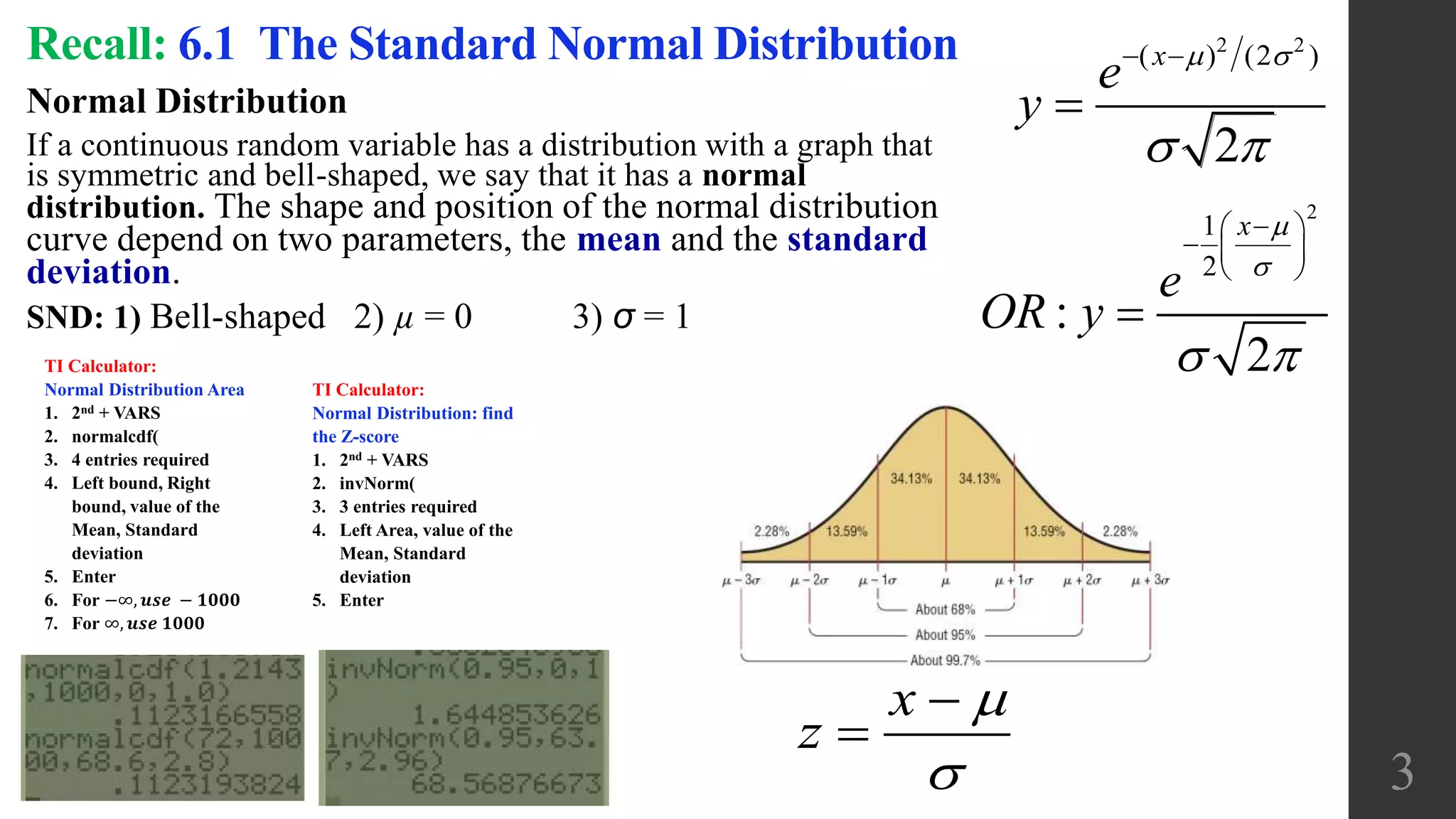
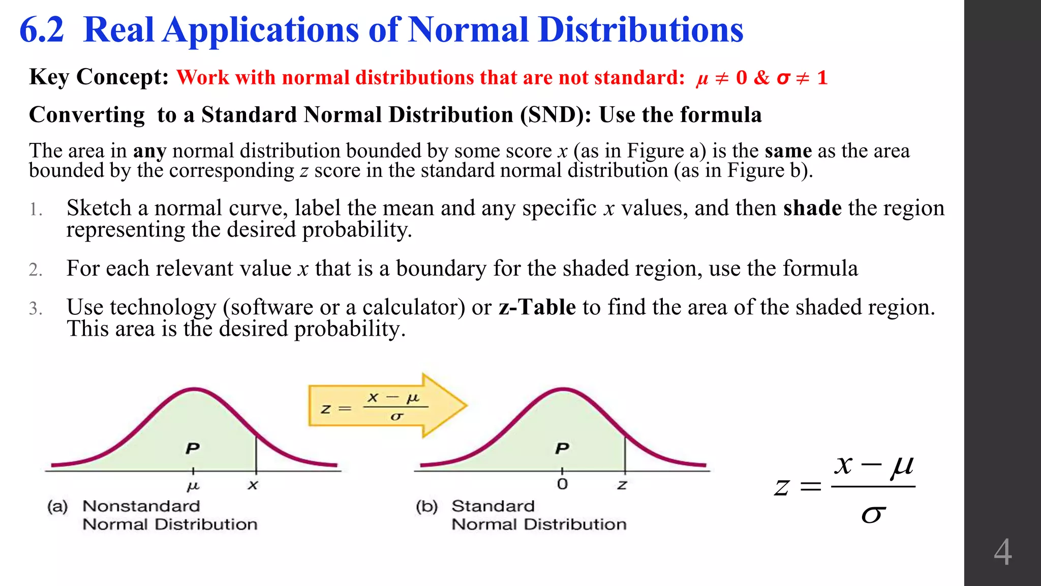
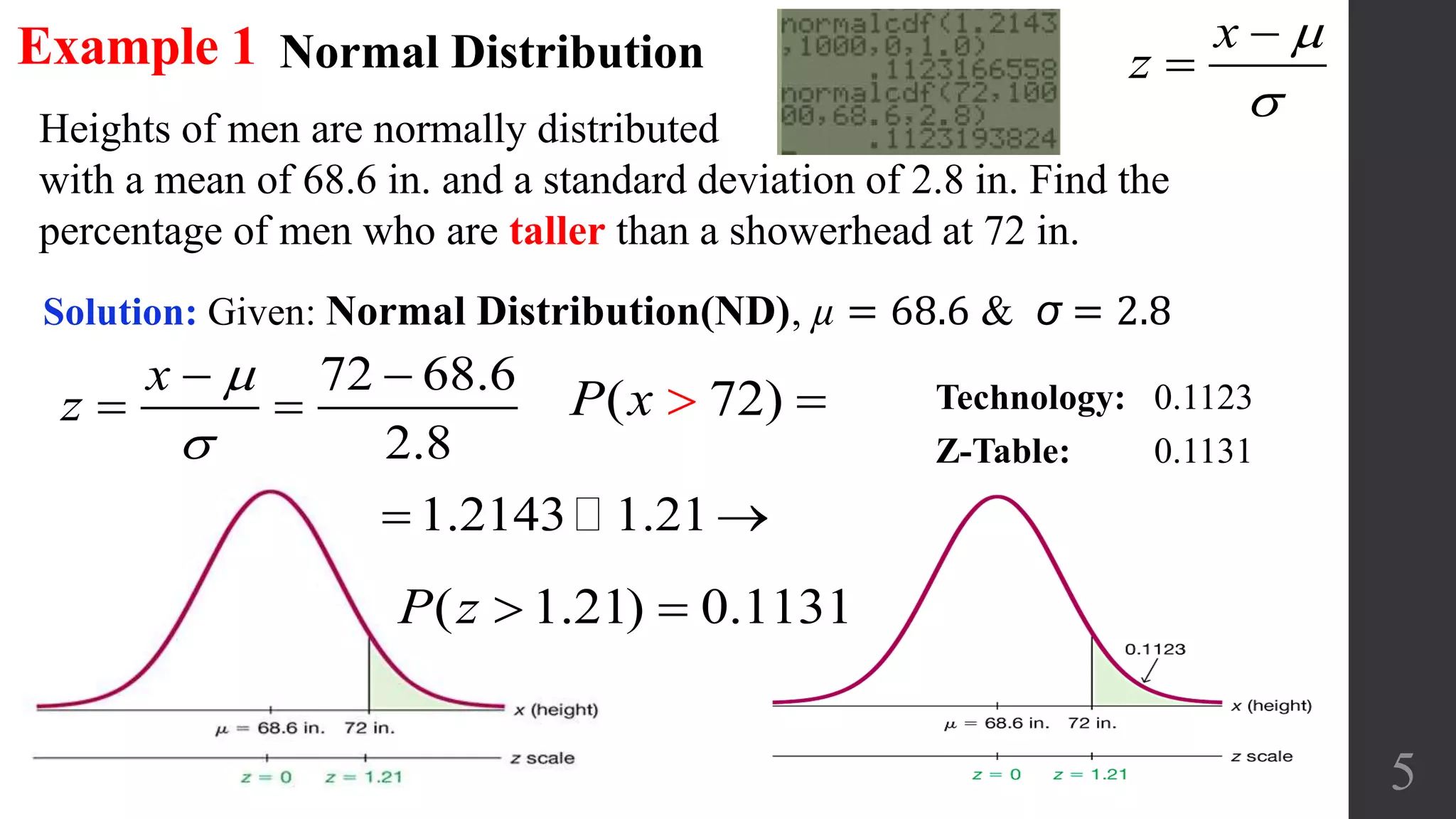
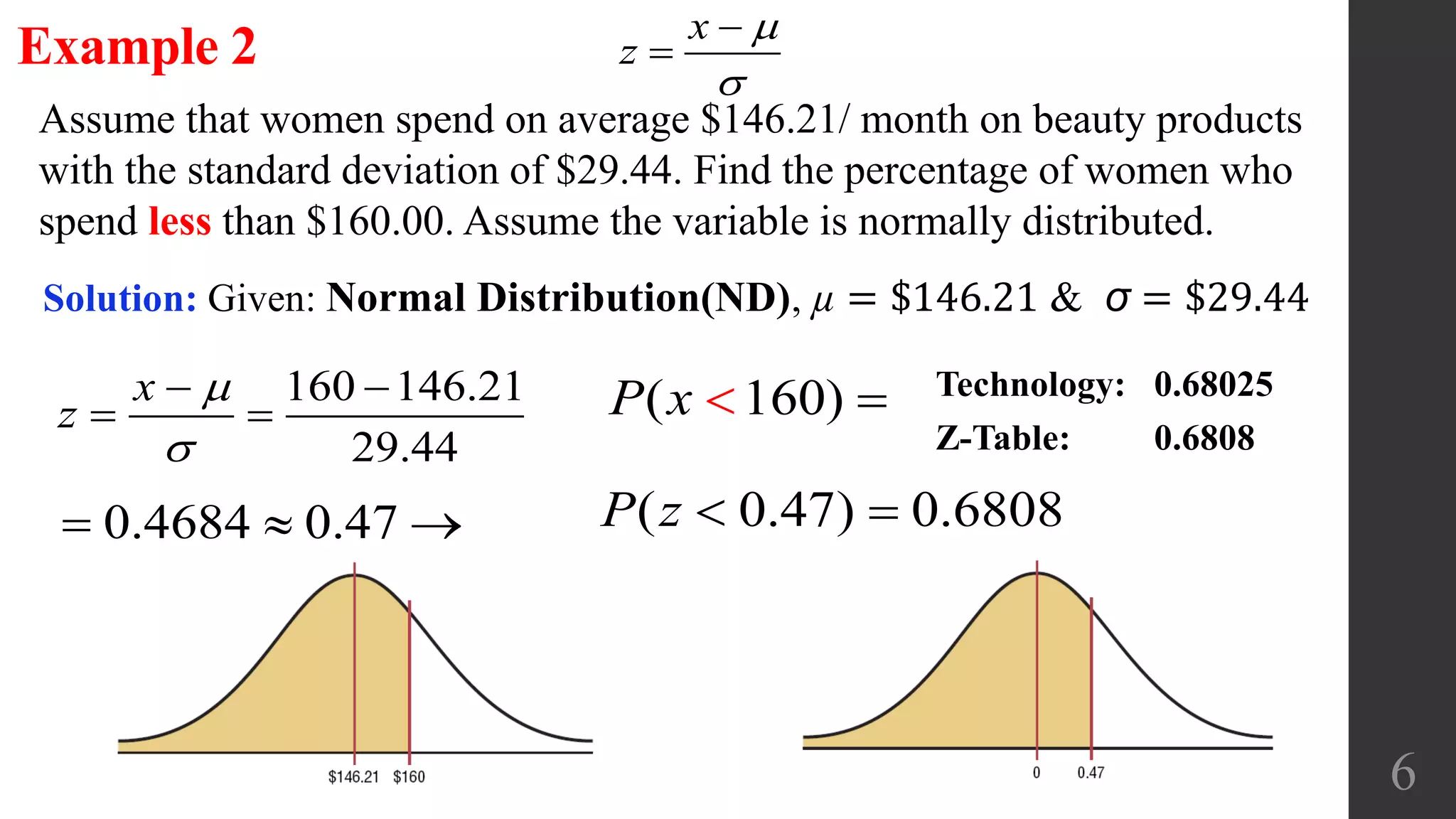
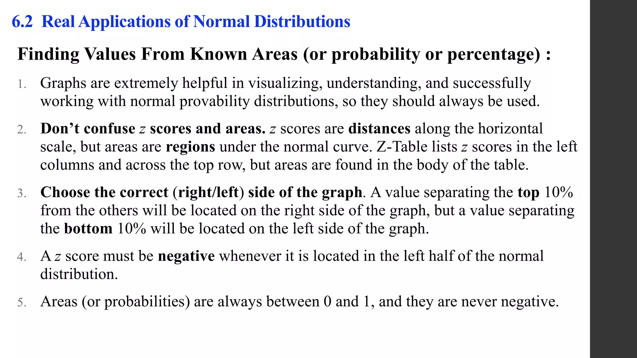
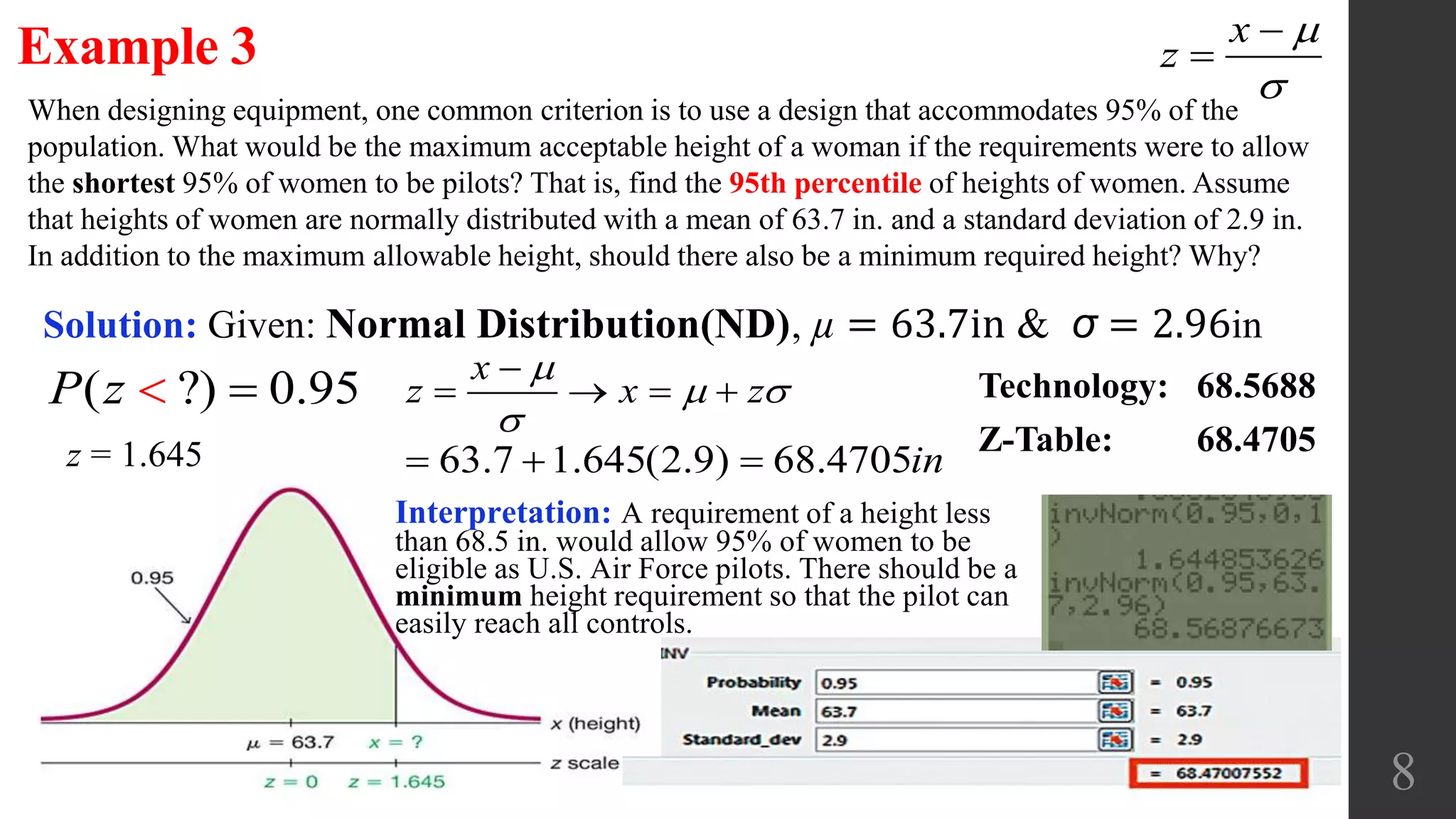
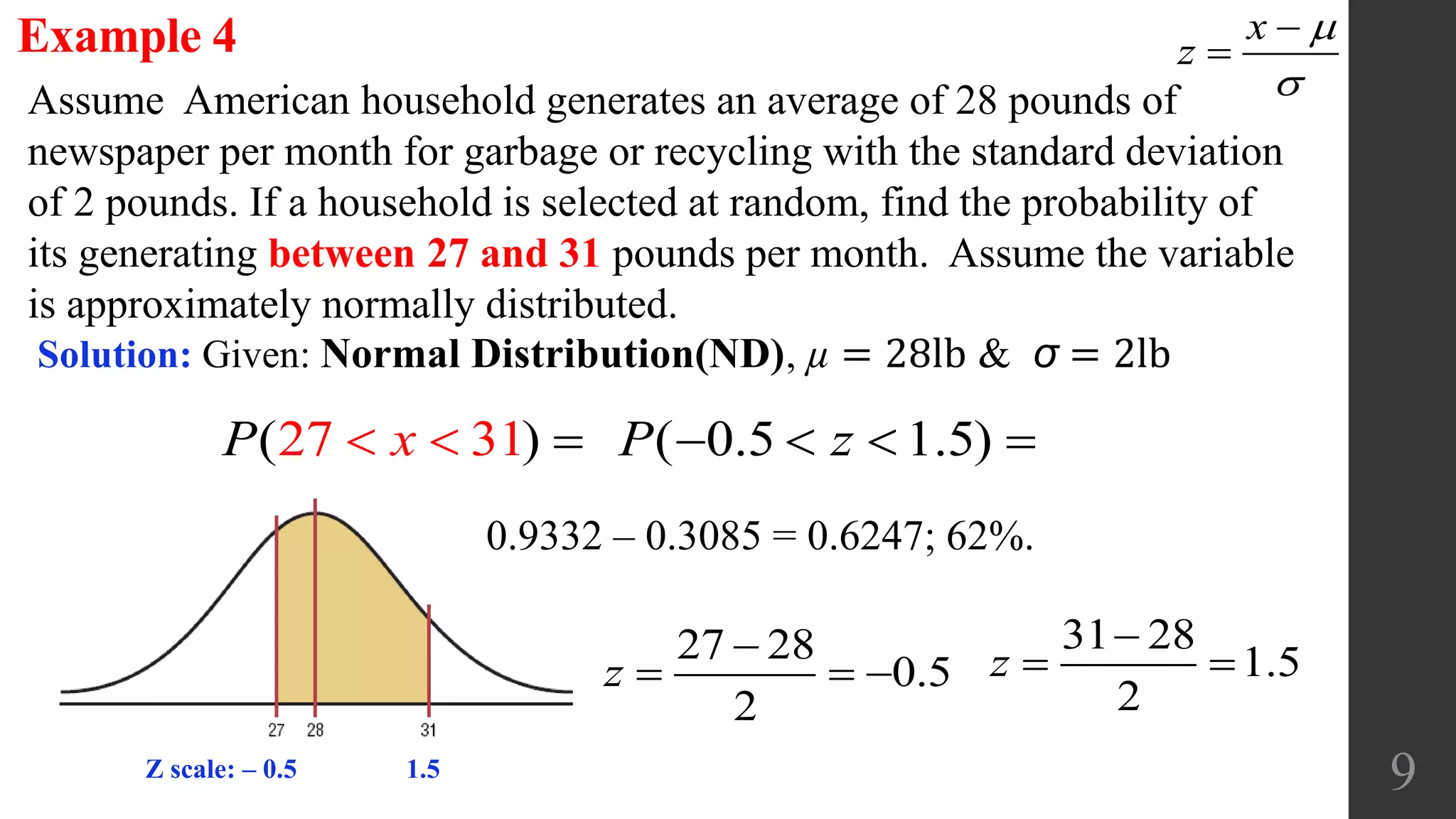
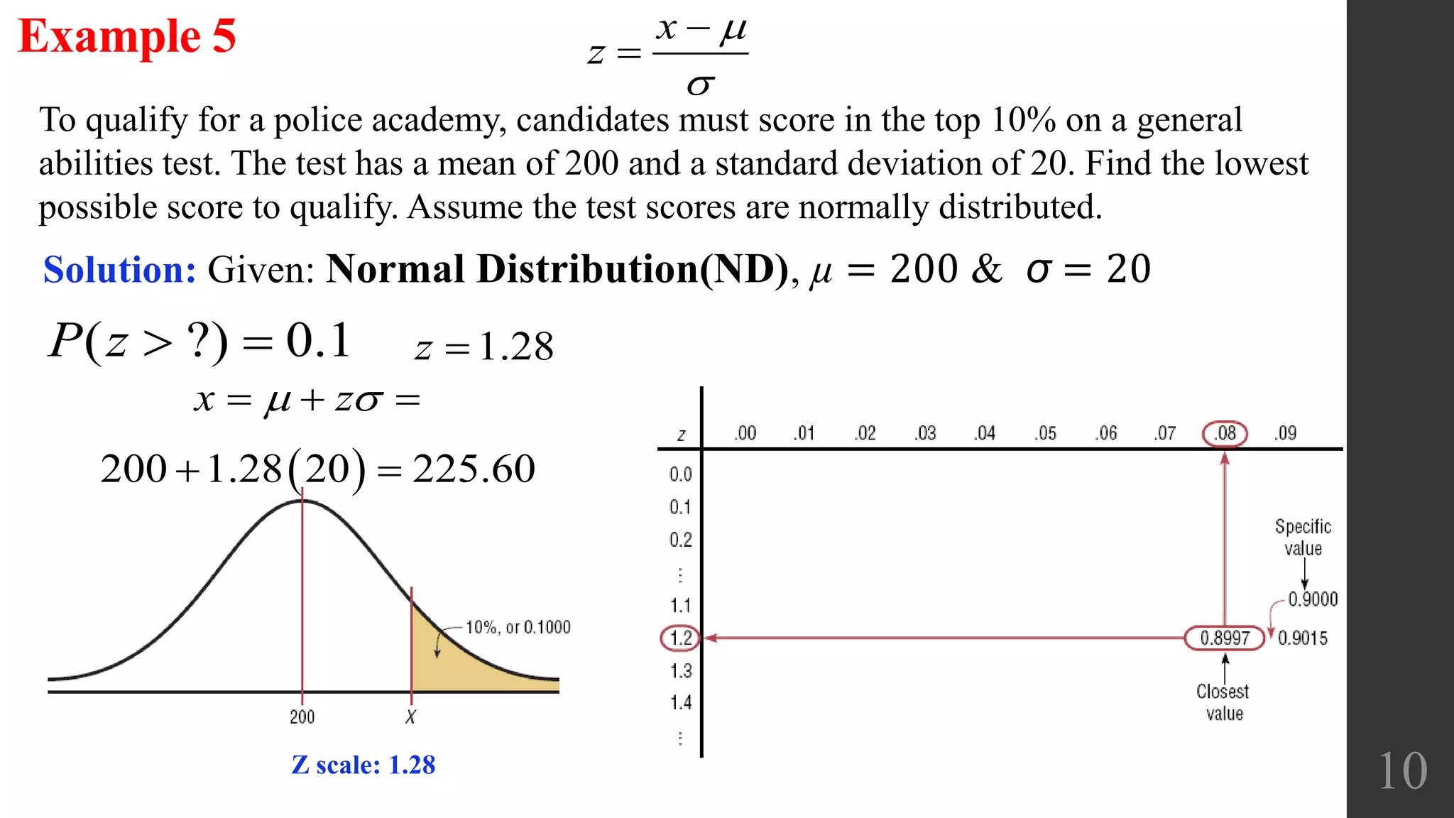
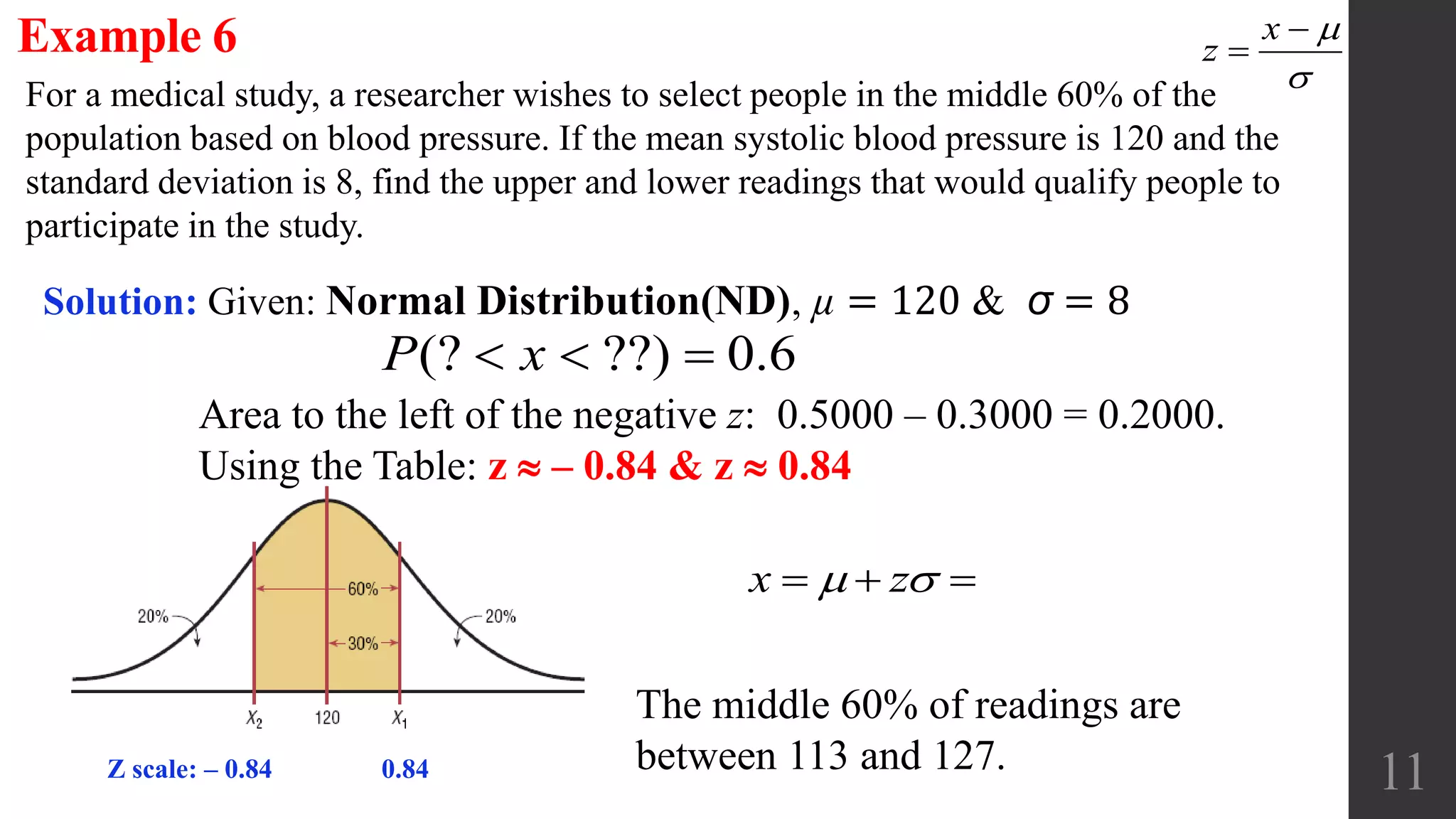
Elementary Statistics
Chapter 6:
Normal Probability
Distributions
6.2 Real Applications
of Normal
Distributions
1
Chapter 6: Normal Probability Distribution
6.1 The Standard Normal Distribution
6.2 Real Applications of Normal Distributions
6.3 Sampling Distributions and Estimators
6.4 The Central Limit Theorem
6.5 Assessing Normality
6.6 Normal as Approximation to Binomial
2
Objectives:
• Identify distributions as symmetric or skewed.
• Identify the properties of a normal distribution.
• Find the area under the standard normal distribution, given various z values.
• Find probabilities for a normally distributed variable by transforming it into a standard normal variable.
• Find specific data values for given percentages, using the standard normal distribution.
• Use the central limit theorem to solve problems involving sample means for large samples.
• Use the normal approximation to compute probabilities for a binomial variable.
Recall: 6.1 The Standard Normal Distribution
Normal Distribution
If a continuous random variable has a distribution with a graph that
is symmetric and bell-shaped, we say that it has a normal
distribution. The shape and position of the normal distribution
curve depend on two parameters, the mean and the standard
deviation.
SND: 1) Bell-shaped 2) µ = 0 3) σ = 1
3
2 2
( ) (2 )
2
x
e
y
 
 
 

2
1
2
:
2
x
e
OR y


 
 
  
 

x
z




TI Calculator:
Normal Distribution Area
1. 2nd + VARS
2. normalcdf(
3. 4 entries required
4. Left bound, Right
bound, value of the
Mean, Standard
deviation
5. Enter
6. For −∞, 𝒖𝒔𝒆 − 𝟏𝟎𝟎𝟎
7. For ∞, 𝒖𝒔𝒆 𝟏𝟎𝟎𝟎
TI Calculator:
Normal Distribution: find
the Z-score
1. 2nd + VARS
2. invNorm(
3. 3 entries required
4. Left Area, value of the
Mean, Standard
deviation
5. Enter
Key Concept: Work with normal distributions that are not standard: µ ≠ 𝟎 & σ ≠ 𝟏
Converting to a Standard Normal Distribution (SND): Use the formula
The area in any normal distribution bounded by some score x (as in Figure a) is the same as the area
bounded by the corresponding z score in the standard normal distribution (as in Figure b).
1. Sketch a normal curve, label the mean and any specific x values, and then shade the region
representing the desired probability.
2. For each relevant value x that is a boundary for the shaded region, use the formula
3. Use technology (software or a calculator) or z-Table to find the area of the shaded region.
This area is the desired probability.
6.2 Real Applications of Normal Distributions
x
z




4
5
Heights of men are normally distributed
with a mean of 68.6 in. and a standard deviation of 2.8 in. Find the
percentage of men who are taller than a showerhead at 72 in.
Example 1 Normal Distribution
Solution: Given: Normal Distribution(ND), µ = 68.6 & σ = 2.8
x
z




72 68.6
2.8
x
z


 
 
1.2143 1.21 
( 1.21) 0.1131P z  
Technology: 0.1123
Z-Table: 0.1131
( 72)P x  
6
Assume that women spend on average $146.21/ month on beauty products
with the standard deviation of $29.44. Find the percentage of women who
spend less than $160.00. Assume the variable is normally distributed.
Example 2
Solution: Given: Normal Distribution(ND), µ = $146.21 & σ = $29.44
x
z




0.4684 0.47   ( 0.47) 0.6808P z  
Technology: 0.68025
Z-Table: 0.6808
160 146.21
29.44
x
z


 
  ( 160)P x  
Finding Values From Known Areas (or probability or percentage) :
1. Graphs are extremely helpful in visualizing, understanding, and successfully
working with normal provability distributions, so they should always be used.
2. Don’t confuse z scores and areas. z scores are distances along the horizontal
scale, but areas are regions under the normal curve. Z-Table lists z scores in the left
columns and across the top row, but areas are found in the body of the table.
3. Choose the correct (right/left) side of the graph. A value separating the top 10%
from the others will be located on the right side of the graph, but a value separating
the bottom 10% will be located on the left side of the graph.
4. A z score must be negative whenever it is located in the left half of the normal
distribution.
5. Areas (or probabilities) are always between 0 and 1, and they are never negative.
6.2 Real Applications of Normal Distributions
8
When designing equipment, one common criterion is to use a design that accommodates 95% of the
population. What would be the maximum acceptable height of a woman if the requirements were to allow
the shortest 95% of women to be pilots? That is, find the 95th percentile of heights of women. Assume
that heights of women are normally distributed with a mean of 63.7 in. and a standard deviation of 2.9 in.
In addition to the maximum allowable height, should there also be a minimum required height? Why?
Example 3
Solution: Given: Normal Distribution(ND), µ = 63.7in & σ = 2.96in
x
z




( ?) 0.95P z  Technology: 68.5688
Z-Table: 68.4705
x
z x z

 


   
z = 1.645 63.7 1.645(2.9) 68.4705in  
Interpretation: A requirement of a height less
than 68.5 in. would allow 95% of women to be
eligible as U.S. Air Force pilots. There should be a
minimum height requirement so that the pilot can
easily reach all controls.
9
Assume American household generates an average of 28 pounds of
newspaper per month for garbage or recycling with the standard deviation
of 2 pounds. If a household is selected at random, find the probability of
its generating between 27 and 31 pounds per month. Assume the variable
is approximately normally distributed.
Example 4
Solution: Given: Normal Distribution(ND), µ = 28lb & σ = 2lb
x
z




1(27 )3xP   
27 28
0.5
2

  z
31 28
1.5
2

 z
( 0.5 1.5)P z   
0.9332 – 0.3085 = 0.6247; 62%.
Z scale: ‒ 0.5 1.5
10
To qualify for a police academy, candidates must score in the top 10% on a general
abilities test. The test has a mean of 200 and a standard deviation of 20. Find the lowest
possible score to qualify. Assume the test scores are normally distributed.
Example 5
Solution: Given: Normal Distribution(ND), µ = 200 & σ = 20
x
z




( ?) 0.1P z  
Z scale: 1.28
1.28z 
x z   
 200 1.28 20 225.60 
11
For a medical study, a researcher wishes to select people in the middle 60% of the
population based on blood pressure. If the mean systolic blood pressure is 120 and the
standard deviation is 8, find the upper and lower readings that would qualify people to
participate in the study.
Example 6
Solution: Given: Normal Distribution(ND), µ = 120 & σ = 8
x
z




(? ??) 0.6P x  
Z scale: ‒ 0.84 0.84
Area to the left of the negative z: 0.5000 – 0.3000 = 0.2000.
Using the Table: z  – 0.84 & z  0.84
The middle 60% of readings are
between 113 and 127.
x z   

Real Applications of Normal Distributions

  • 1.
    Elementary Statistics Chapter 6: NormalProbability Distributions 6.2 Real Applications of Normal Distributions 1
  • 2.
    Chapter 6: NormalProbability Distribution 6.1 The Standard Normal Distribution 6.2 Real Applications of Normal Distributions 6.3 Sampling Distributions and Estimators 6.4 The Central Limit Theorem 6.5 Assessing Normality 6.6 Normal as Approximation to Binomial 2 Objectives: • Identify distributions as symmetric or skewed. • Identify the properties of a normal distribution. • Find the area under the standard normal distribution, given various z values. • Find probabilities for a normally distributed variable by transforming it into a standard normal variable. • Find specific data values for given percentages, using the standard normal distribution. • Use the central limit theorem to solve problems involving sample means for large samples. • Use the normal approximation to compute probabilities for a binomial variable.
  • 3.
    Recall: 6.1 TheStandard Normal Distribution Normal Distribution If a continuous random variable has a distribution with a graph that is symmetric and bell-shaped, we say that it has a normal distribution. The shape and position of the normal distribution curve depend on two parameters, the mean and the standard deviation. SND: 1) Bell-shaped 2) µ = 0 3) σ = 1 3 2 2 ( ) (2 ) 2 x e y        2 1 2 : 2 x e OR y             x z     TI Calculator: Normal Distribution Area 1. 2nd + VARS 2. normalcdf( 3. 4 entries required 4. Left bound, Right bound, value of the Mean, Standard deviation 5. Enter 6. For −∞, 𝒖𝒔𝒆 − 𝟏𝟎𝟎𝟎 7. For ∞, 𝒖𝒔𝒆 𝟏𝟎𝟎𝟎 TI Calculator: Normal Distribution: find the Z-score 1. 2nd + VARS 2. invNorm( 3. 3 entries required 4. Left Area, value of the Mean, Standard deviation 5. Enter
  • 4.
    Key Concept: Workwith normal distributions that are not standard: µ ≠ 𝟎 & σ ≠ 𝟏 Converting to a Standard Normal Distribution (SND): Use the formula The area in any normal distribution bounded by some score x (as in Figure a) is the same as the area bounded by the corresponding z score in the standard normal distribution (as in Figure b). 1. Sketch a normal curve, label the mean and any specific x values, and then shade the region representing the desired probability. 2. For each relevant value x that is a boundary for the shaded region, use the formula 3. Use technology (software or a calculator) or z-Table to find the area of the shaded region. This area is the desired probability. 6.2 Real Applications of Normal Distributions x z     4
  • 5.
    5 Heights of menare normally distributed with a mean of 68.6 in. and a standard deviation of 2.8 in. Find the percentage of men who are taller than a showerhead at 72 in. Example 1 Normal Distribution Solution: Given: Normal Distribution(ND), µ = 68.6 & σ = 2.8 x z     72 68.6 2.8 x z       1.2143 1.21  ( 1.21) 0.1131P z   Technology: 0.1123 Z-Table: 0.1131 ( 72)P x  
  • 6.
    6 Assume that womenspend on average $146.21/ month on beauty products with the standard deviation of $29.44. Find the percentage of women who spend less than $160.00. Assume the variable is normally distributed. Example 2 Solution: Given: Normal Distribution(ND), µ = $146.21 & σ = $29.44 x z     0.4684 0.47   ( 0.47) 0.6808P z   Technology: 0.68025 Z-Table: 0.6808 160 146.21 29.44 x z       ( 160)P x  
  • 7.
    Finding Values FromKnown Areas (or probability or percentage) : 1. Graphs are extremely helpful in visualizing, understanding, and successfully working with normal provability distributions, so they should always be used. 2. Don’t confuse z scores and areas. z scores are distances along the horizontal scale, but areas are regions under the normal curve. Z-Table lists z scores in the left columns and across the top row, but areas are found in the body of the table. 3. Choose the correct (right/left) side of the graph. A value separating the top 10% from the others will be located on the right side of the graph, but a value separating the bottom 10% will be located on the left side of the graph. 4. A z score must be negative whenever it is located in the left half of the normal distribution. 5. Areas (or probabilities) are always between 0 and 1, and they are never negative. 6.2 Real Applications of Normal Distributions
  • 8.
    8 When designing equipment,one common criterion is to use a design that accommodates 95% of the population. What would be the maximum acceptable height of a woman if the requirements were to allow the shortest 95% of women to be pilots? That is, find the 95th percentile of heights of women. Assume that heights of women are normally distributed with a mean of 63.7 in. and a standard deviation of 2.9 in. In addition to the maximum allowable height, should there also be a minimum required height? Why? Example 3 Solution: Given: Normal Distribution(ND), µ = 63.7in & σ = 2.96in x z     ( ?) 0.95P z  Technology: 68.5688 Z-Table: 68.4705 x z x z          z = 1.645 63.7 1.645(2.9) 68.4705in   Interpretation: A requirement of a height less than 68.5 in. would allow 95% of women to be eligible as U.S. Air Force pilots. There should be a minimum height requirement so that the pilot can easily reach all controls.
  • 9.
    9 Assume American householdgenerates an average of 28 pounds of newspaper per month for garbage or recycling with the standard deviation of 2 pounds. If a household is selected at random, find the probability of its generating between 27 and 31 pounds per month. Assume the variable is approximately normally distributed. Example 4 Solution: Given: Normal Distribution(ND), µ = 28lb & σ = 2lb x z     1(27 )3xP    27 28 0.5 2    z 31 28 1.5 2   z ( 0.5 1.5)P z    0.9332 – 0.3085 = 0.6247; 62%. Z scale: ‒ 0.5 1.5
  • 10.
    10 To qualify fora police academy, candidates must score in the top 10% on a general abilities test. The test has a mean of 200 and a standard deviation of 20. Find the lowest possible score to qualify. Assume the test scores are normally distributed. Example 5 Solution: Given: Normal Distribution(ND), µ = 200 & σ = 20 x z     ( ?) 0.1P z   Z scale: 1.28 1.28z  x z     200 1.28 20 225.60 
  • 11.
    11 For a medicalstudy, a researcher wishes to select people in the middle 60% of the population based on blood pressure. If the mean systolic blood pressure is 120 and the standard deviation is 8, find the upper and lower readings that would qualify people to participate in the study. Example 6 Solution: Given: Normal Distribution(ND), µ = 120 & σ = 8 x z     (? ??) 0.6P x   Z scale: ‒ 0.84 0.84 Area to the left of the negative z: 0.5000 – 0.3000 = 0.2000. Using the Table: z  – 0.84 & z  0.84 The middle 60% of readings are between 113 and 127. x z   