More Related Content
PPT

PPT
The Normal Distribution.ppt 
PPTX

PPTX
Probability, Normal Distribution and Z-Scores.pptx 
PDF

PPT
continuous probability distributions.ppt 
PPT

PPT
Binomeal Distribution Silde, Prileminary Knowledge Similar to chapter_6_modified_slides_0_222222222222222222222222.ppt

PPT

PDF

PPTX
Statistics_further_00 Normal Distribution.pptx 
PPT
A Level Mathematics Normal distributions.ppt 
PPT
Gausian Distribution lecture one in details.ppt 
PPTX
Inferiential statistics .pptx 
PPTX
Real Applications of Normal Distributions 
PPT
normal distribtion best lecture series.ppt 
PPTX
The Standard Normal Distribution 
PDF
Module 6 - Continuous Distribution_efcd52595b081d24a9bc3ca31b5f8d05.pdf 
PPT
Statistik 1 6 distribusi probabilitas normal 
PPT
normal-distribution-2.ppt 
PPT
Business Statistics Chapter 6 
PPTX
Chapter 2 normal distribution grade 11 ppt 
PPT

PPTX
Lecture 6 Normal Distribution.pptx 
PDF
MAT225-Ch 6 (Normal Distribution)HGFF.pdf 
PPTX
Real Applications of Normal Distributions 
PPT
-Normal-Distribution-ppt.ppt-POWER PRESENTATION ON STATISTICS AND PROBABILITY 
PPTX
Using the normal table in reverse for any normal variable x More from MarjorieMalveda2

PPTX
1111111111111111111111111111111111111111111(1).pptx 
PPTX
1111111111111111111111111111111111111111111111pli.pptx 
PPT
chapter_11_0000000000000000000000000000000000.ppt 
PPT
2_2018_12_16!09_51_48_AMmmmmmmmmmmmmmmmmmm.ppt 
PPT
1582765776-Lecture9999999999999999999999999999.ppt 
PPT
PP07777777777777777777777777777777777.ppt 
PPT
333333333333333333333333333_Complete.ppt 
PPT
Chapter-088888888888888888888888888888 (1).ppt 
PPT
121243255555555555555555555555555ptest.ppt 
PPT
250Lec5Fall111111111111111111111111111111111113.ppt 
PPTX
bgghvghvfcxfdx98787877666555555555555ghgv [.pptx 
PPT
Gerstmannnnnnnnnnnnnnnnnnnnnnnnnnnnnnnnnnnnnnnn_PP09.ppt 
PPT
sumstatssssssssssssssssssssssssssssssssss.ppt 
PPTX
Normal Distribution- Fundamentals and Using Distributions - Lesson.pptx 
PPT
Chapter 4444444444444444444444444444444444.ppt 
PPTX
Standard Deviation and Variance - Lesson.pptx 
PPTX
S1-Chp2-MeasuresOfLocationAndSpread.pptx 
PPT
sumstatsssssssssssssssssssssssssssssssss.ppt 
PPT
1582765776-Lecture999999999999999999.ppt 
PPT
discrete_259_2007 (2)222222222222222.ppt Recently uploaded

PPTX
Lesson_1 Acceleration.pptx_Science 8-4th quarter 
PDF
Using T-Test to Analyze Research Data.pdf 
PPTX
MEMORY &FORGETTING. Shilpa Hotakar.Psychology pptx 
PDF
operation with integers and finding common ground worksheet solutions/7th cla... 
PDF
Chapter 05 Drugs Acting on the Central Nervous System: Anticonvulsant (Antiep... 
PPTX
A detailed notes on Conjugate Vaccine and its mechanism. 
PDF
RAJAT ARORA SIR PHYSICAL EDUCATION NOTES ALL CHAPTERS .pdf 
PDF
RAIN, BMP, CURRENT, ESP 32, GAS, LINE, IR, JOYSTICK, LCD, LM35, SD, MOTION, P... 
PPTX
Chapter 1 - Introduction to Business Research.pptx 
PDF
APPSC APPSC AEE-AE GENERAL STUDIES QUESTION PAPER.pdf 
PDF
APPSC APPSC Forest Draughtsman GS Question paper.pdf 
PDF
Why Projects Fail – The Need to “Do the Right Project” and “Do the Project Ri... 
PPTX
EYE IRRIGATION AND INSTILLATION....pptx 
PPTX
How Physician Assistants in the USA Earn CME Credits Online.pptx 
PPTX
SOLAR SYSTEM.pptx || The infinity solar system 
PDF
West Hatch High School - GCSE Media Specification 
PDF
Chapter 05 Drugs Acting on the Central Nervous System: Anti-Depressant Drugs 
PPT
West Hatch High School - GCSE History Option 
PPTX
How to Manage Closest Location in Odoo 18 Inventory 
PPTX
Chapter 1: Introduction to Economics - Macroeconomics and Microeconomics.pptx chapter_6_modified_slides_0_222222222222222222222222.ppt
- 1.
Copyright © 2016Pearson Education, Ltd. Chapter 6, Slide 1
The Normal
Distribution
Chapter 6
- 2.
Copyright © 2016Pearson Education, Ltd. Chapter 6, Slide 2
Objectives
In this chapter, you learn:
To compute probabilities from the normal distribution
How to use the normal distribution to solve business
problems
To use the normal probability plot to determine whether
a set of data is approximately normally distributed
- 3.
Copyright © 2016Pearson Education, Ltd. Chapter 6, Slide 3
Continuous Probability Distributions
A continuous variable is a variable that can
assume any value on a continuum (can assume
an uncountable number of values)
thickness of an item
time required to complete a task
temperature of a solution
height, in inches
These can potentially take on any value
depending only on the ability to precisely and
accurately measure
- 4.
Copyright © 2016Pearson Education, Ltd. Chapter 6, Slide 4
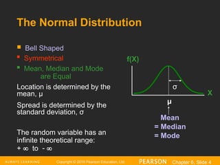
Bell Shaped
Symmetrical
Mean, Median and Mode
are Equal
Location is determined by the
mean, μ
Spread is determined by the
standard deviation, σ
The random variable has an
infinite theoretical range:
+ to
Mean
= Median
= Mode
X
f(X)
μ
σ
The Normal Distribution
- 5.
Copyright © 2016Pearson Education, Ltd. Chapter 6, Slide 5
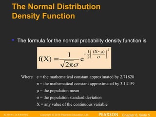
The Normal Distribution
Density Function
2
μ)
(X
2
1
e
2π
1
f(X)
The formula for the normal probability density function is
Where e = the mathematical constant approximated by 2.71828
π = the mathematical constant approximated by 3.14159
μ = the population mean
σ = the population standard deviation
X = any value of the continuous variable
- 6.
Copyright © 2016Pearson Education, Ltd. Chapter 6, Slide 6
A
B
C
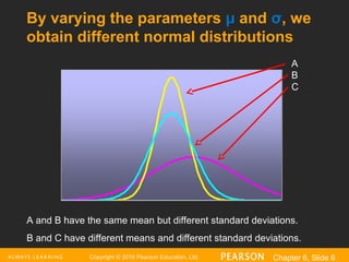
A and B have the same mean but different standard deviations.
B and C have different means and different standard deviations.
By varying the parameters μ and σ, we
obtain different normal distributions
- 7.
Copyright © 2016Pearson Education, Ltd. Chapter 6, Slide 7
The Normal Distribution Shape
X
f(X)
μ
σ
Changing μ shifts the
distribution left or right.
Changing σ increases
or decreases the
spread.
- 8.
Copyright © 2016Pearson Education, Ltd. Chapter 6, Slide 8
The Standardized Normal
Any normal distribution (with any mean and
standard deviation combination) can be
transformed into the standardized normal
distribution (Z)
To compute normal probabilities need to
transform X units into Z units
The standardized normal distribution (Z) has a
mean of 0 and a standard deviation of 1
- 9.
Copyright © 2016Pearson Education, Ltd. Chapter 6, Slide 9
Translation to the Standardized
Normal Distribution
Translate from X to the standardized normal
(the “Z” distribution) by subtracting the mean
of X and dividing by its standard deviation:
σ
μ
X
Z
The Z distribution always has mean = 0 and
standard deviation = 1
- 10.
Copyright © 2016Pearson Education, Ltd. Chapter 6, Slide 10
The Standardized Normal
Probability Density Function
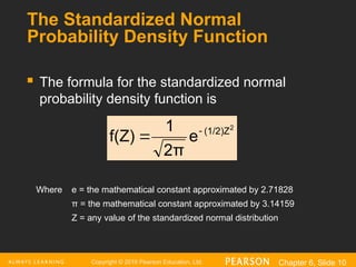
The formula for the standardized normal
probability density function is
Where e = the mathematical constant approximated by 2.71828
π = the mathematical constant approximated by 3.14159
Z = any value of the standardized normal distribution
2
(1/2)Z
e
2π
1
f(Z)
- 11.
Copyright © 2016Pearson Education, Ltd. Chapter 6, Slide 11
The Standardized
Normal Distribution
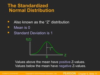
Also known as the “Z” distribution
Mean is 0
Standard Deviation is 1
Z
f(Z)
0
1
Values above the mean have positive Z-values.
Values below the mean have negative Z-values.
- 12.
Copyright © 2016Pearson Education, Ltd. Chapter 6, Slide 12
Example
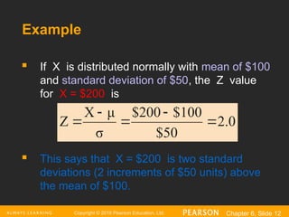
If X is distributed normally with mean of $100
and standard deviation of $50, the Z value
for X = $200 is
This says that X = $200 is two standard
deviations (2 increments of $50 units) above
the mean of $100.
2.0
$50
100
$
$200
σ
μ
X
Z
- 13.
Copyright © 2016Pearson Education, Ltd. Chapter 6, Slide 13
Comparing X and Z units
Note that the shape of the distribution is the same,
only the scale has changed. We can express the
problem in the original units (X in dollars) or in
standardized units (Z)
Z
$100
2.0
0
$200 $X(μ = $100, σ = $50)
(μ = 0, σ = 1)
- 14.
Copyright © 2016Pearson Education, Ltd. Chapter 6, Slide 14
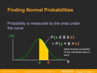
Probability is measured by the area under
the curve
a b X
f(X)
P a X b
( )
≤
≤
P a X b
( )
<
<
=
(Note that the probability
of any individual value is
zero)
Finding Normal Probabilities
- 15.
Copyright © 2016Pearson Education, Ltd. Chapter 6, Slide 15
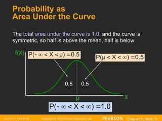
Probability as
Area Under the Curve
The total area under the curve is 1.0, and the curve is
symmetric, so half is above the mean, half is below
f(X)
X
μ
0.5
0.5
1.0
)
X
P(
0.5
)
X
P(μ
0.5
μ)
X
P(
- 16.
Copyright © 2016Pearson Education, Ltd. Chapter 6, Slide 16
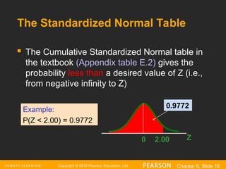
The Standardized Normal Table
The Cumulative Standardized Normal table in
the textbook (Appendix table E.2) gives the
probability less than a desired value of Z (i.e.,
from negative infinity to Z)
Z
0 2.00
0.9772
Example:
P(Z < 2.00) = 0.9772
- 17.
Copyright © 2016Pearson Education, Ltd. Chapter 6, Slide 17
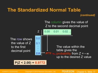
The Standardized Normal Table
The value within the
table gives the
probability from Z =
up to the desired Z value
.9772
2.0
P(Z < 2.00) = 0.9772
The row shows
the value of Z
to the first
decimal point
The column gives the value of
Z to the second decimal point
2.0
.
.
.
(continued)
Z 0.00 0.01 0.02 …
0.0
0.1
- 18.
Copyright © 2016Pearson Education, Ltd. Chapter 6, Slide 18
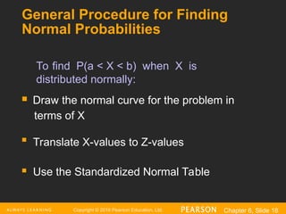
General Procedure for Finding
Normal Probabilities
Draw the normal curve for the problem in
terms of X
Translate X-values to Z-values
Use the Standardized Normal Table
To find P(a < X < b) when X is
distributed normally:
- 19.
Copyright © 2016Pearson Education, Ltd. Chapter 6, Slide 19
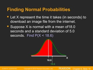
Finding Normal Probabilities
Let X represent the time it takes (in seconds) to
download an image file from the internet.
Suppose X is normal with a mean of18.0
seconds and a standard deviation of 5.0
seconds. Find P(X < 18.6)
18.6
X
18.0
- 20.
Copyright © 2016Pearson Education, Ltd. Chapter 6, Slide 20
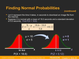
Finding Normal Probabilities
Let X represent the time it takes, in seconds to download an image file from
the internet.
Suppose X is normal with a mean of 18.0 seconds and a standard deviation
of 5.0 seconds. Find P(X < 18.6)
Z
0.12
0
X
18.6
18
μ = 18
σ = 5
μ = 0
σ = 1
(continued)
0.12
5.0
8.0
1
18.6
σ
μ
X
Z
P(X < 18.6) P(Z < 0.12)
- 21.
Copyright © 2016Pearson Education, Ltd. Chapter 6, Slide 21
Z
0.12
0.5478
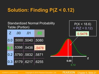
Standardized Normal Probability
Table (Portion)
0.00
= P(Z < 0.12)
P(X < 18.6)
Z .00 .01
0.0 .5000 .5040 .5080
.5398 .5438
0.2 .5793 .5832 .5871
0.3 .6179 .6217 .6255
.02
0.1 .5478
Solution: Finding P(Z < 0.12)
- 22.
Copyright © 2016Pearson Education, Ltd. Chapter 6, Slide 22
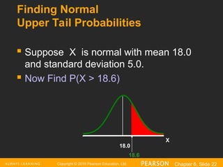
Finding Normal
Upper Tail Probabilities
Suppose X is normal with mean 18.0
and standard deviation 5.0.
Now Find P(X > 18.6)
X
18.6
18.0
- 23.
Copyright © 2016Pearson Education, Ltd. Chapter 6, Slide 23
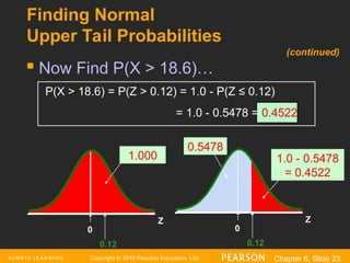
Finding Normal
Upper Tail Probabilities
Now Find P(X > 18.6)…
(continued)
Z
0.12
0
Z
0.12
0.5478
0
1.000 1.0 - 0.5478
= 0.4522
P(X > 18.6) = P(Z > 0.12) = 1.0 - P(Z ≤ 0.12)
= 1.0 - 0.5478 = 0.4522
- 24.
Copyright © 2016Pearson Education, Ltd. Chapter 6, Slide 24
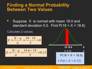
Finding a Normal Probability
Between Two Values
Suppose X is normal with mean 18.0 and
standard deviation 5.0. Find P(18 < X < 18.6)
P(18 < X < 18.6)
= P(0 < Z < 0.12)
Z
0.12
0
X
18.6
18
0
5
8
1
18
σ
μ
X
Z
0.12
5
8
1
18.6
σ
μ
X
Z
Calculate Z-values:
- 25.
Copyright © 2016Pearson Education, Ltd. Chapter 6, Slide 25
Z
0.12
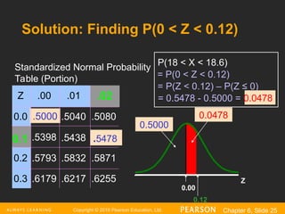
0.0478
0.00
= P(0 < Z < 0.12)
P(18 < X < 18.6)
= P(Z < 0.12) – P(Z ≤ 0)
= 0.5478 - 0.5000 = 0.0478
0.5000
Z .00 .01
0.0 .5000 .5040 .5080
.5398 .5438
0.2 .5793 .5832 .5871
0.3 .6179 .6217 .6255
.02
0.1 .5478
Standardized Normal Probability
Table (Portion)
Solution: Finding P(0 < Z < 0.12)
- 26.
Copyright © 2016Pearson Education, Ltd. Chapter 6, Slide 26
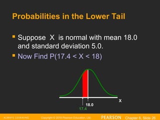
Probabilities in the Lower Tail
Suppose X is normal with mean 18.0
and standard deviation 5.0.
Now Find P(17.4 < X < 18)
X
17.4
18.0
- 27.
Copyright © 2016Pearson Education, Ltd. Chapter 6, Slide 27
Probabilities in the Lower Tail
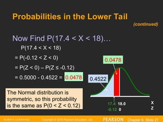
Now Find P(17.4 < X < 18)…
X
17.4 18.0
P(17.4 < X < 18)
= P(-0.12 < Z < 0)
= P(Z < 0) – P(Z ≤ -0.12)
= 0.5000 - 0.4522 = 0.0478
(continued)
0.0478
0.4522
Z
-0.12 0
The Normal distribution is
symmetric, so this probability
is the same as P(0 < Z < 0.12)
- 28.
Copyright © 2016Pearson Education, Ltd. Chapter 6, Slide 28
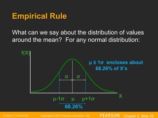
Empirical Rule
μ ± 1σ encloses about
68.26% of X’s
f(X)
X
μ μ+1σ
μ-1σ
What can we say about the distribution of values
around the mean? For any normal distribution:
σ
σ
68.26%
- 29.
Copyright © 2016Pearson Education, Ltd. Chapter 6, Slide 29
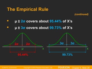
The Empirical Rule
μ ± 2σ covers about 95.44% of X’s
μ ± 3σ covers about 99.73% of X’s
x
μ
2σ 2σ
x
μ
3σ 3σ
95.44% 99.73%
(continued)
- 30.
Copyright © 2016Pearson Education, Ltd. Chapter 6, Slide 30
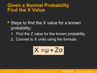
Given a Normal Probability
Find the X Value
Steps to find the X value for a known
probability:
1. Find the Z value for the known probability
2. Convert to X units using the formula:
Zσ
μ
X
- 31.
Copyright © 2016Pearson Education, Ltd. Chapter 6, Slide 31
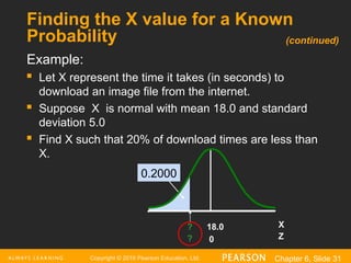
Finding the X value for a Known
Probability
Example:
Let X represent the time it takes (in seconds) to
download an image file from the internet.
Suppose X is normal with mean 18.0 and standard
deviation 5.0
Find X such that 20% of download times are less than
X.
X
? 18.0
0.2000
Z
? 0
(continued)
- 32.
Copyright © 2016Pearson Education, Ltd. Chapter 6, Slide 32
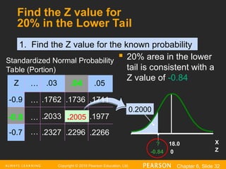
Find the Z value for
20% in the Lower Tail
20% area in the lower
tail is consistent with a
Z value of -0.84
Z .03
-0.9 .1762 .1736
.2033
-0.7 .2327 .2296
.04
-0.8 .2005
Standardized Normal Probability
Table (Portion)
.05
.1711
.1977
.2266
…
…
…
…
X
? 18.0
0.2000
Z
-0.84 0
1. Find the Z value for the known probability
- 33.
Copyright © 2016Pearson Education, Ltd. Chapter 6, Slide 33
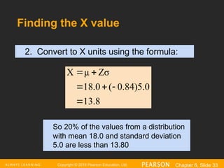
Finding the X value
2. Convert to X units using the formula:
8
.
13
0
.
5
)
84
.
0
(
0
.
18
Zσ
μ
X
So 20% of the values from a distribution
with mean 18.0 and standard deviation
5.0 are less than 13.80
- 34.
Copyright © 2016Pearson Education, Ltd. Chapter 6, Slide 34
Chapter Summary
In this chapter we discussed:
Computing probabilities from the normal distribution
Using the normal distribution to solve business
problems
Using the normal probability plot to determine whether a
set of data is approximately normally distributed