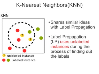
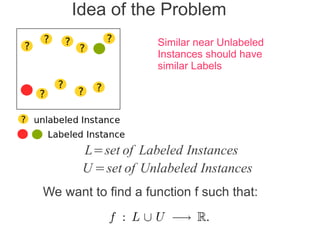
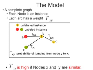
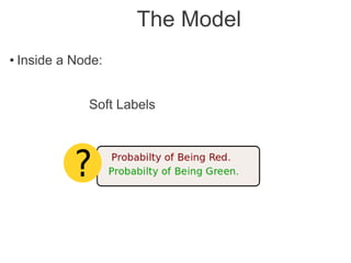
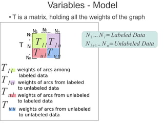
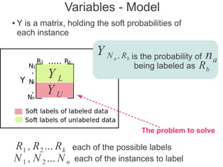
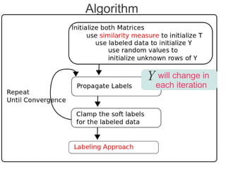
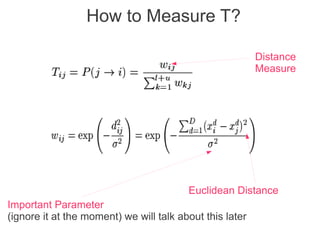
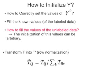
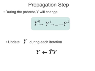
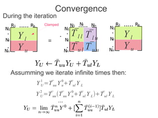
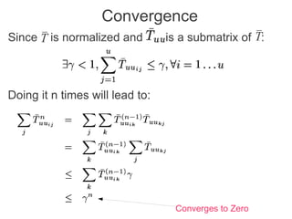
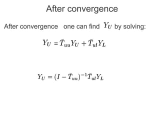
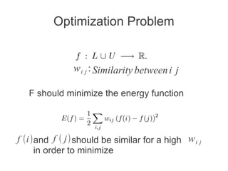
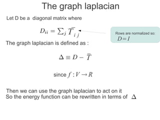
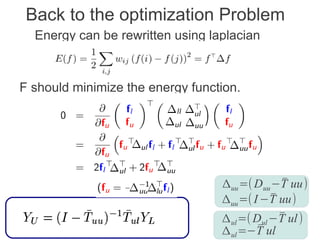
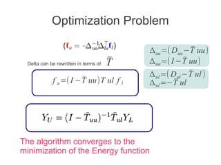
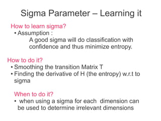
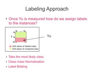
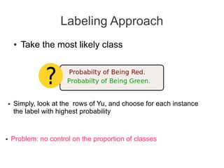
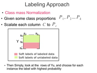
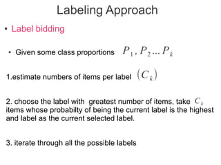
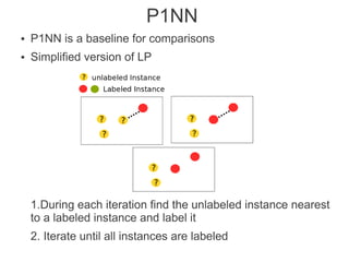
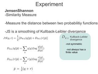
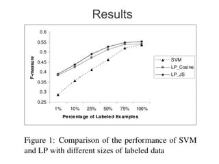
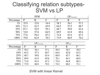
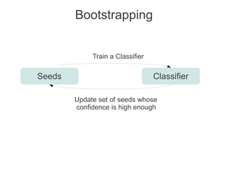
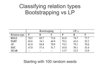
Label propagation is a semi-supervised learning algorithm that propagates labels from a small set of labeled data points to unlabeled data points. The algorithm constructs a graph with nodes for each data point and weighted edges representing similarity between points. It then iteratively propagates the labels across the graph from labeled to unlabeled points until convergence, resulting in "soft" probabilistic labels for all points. The algorithm aims to minimize an energy function that encourages points connected by strong edges to receive similar labels. It performs well with limited labeled data by leveraging the graph structure to make predictions for unlabeled points.

1. Label Propagation
Seminar:
Semi-supervised and unsupervised learning with Applications to NLP
David Przybilla
davida@coli.uni-saarland.de

2. Outline
● What is Label Propagation
● The Algorithm
● The motivation behind the algorithm
● Parameters of Label Propagation
● Relation Extraction with Label Propagation

3. Label Propagation
● Semi-supervised
● Shows good results when the amount of
annotated data is low with respect to the
supervised options
● Similar to kNN

4. K-Nearest Neighbors(KNN)
● Shares similar ideas
with Label Propagation
● Label Propagation
(LP) uses unlabeled
instances during the
process of finding out
the labels

5. Idea of the Problem
Similar near Unlabeled
Instances should have
similar Labels
L=set of Labeled Instances
U =set of Unlabeled Instances
We want to find a function f such that:

6. The Model
● A complete graph
● Each Node is an instance
●
Each arc has a weight T xy
● T xy is high if Nodes x and y are similar.

7. The Model
● Inside a Node:
Soft Labels

8. Variables - Model
● T is a matrix, holding all the weights of the graph
N 1 ... N l = Labeled Data
TllTlu N l+1 .. N n=Unlabeled Data
T u lT u u
Tll
Tlu
T ul
T uu

9. Variables - Model
● Y is a matrix, holding the soft probabilities of
each instance
YN a n
, R b is the probability of a
being labeled as R b
YL
YU
The problem to solve
R1 , R 2 ... R k each of the possible labels
N 1 , N 2 ... N n each of the instances to label

10. Algorithm
Y will change in
each iteration

11. How to Measure T?
Distance
Measure
Euclidean Distance
Important Parameter
(ignore it at the moment) we will talk about this later

12. How to Initialize Y?
0
● How to Correctly set the values of Y ?
● Fill the known values (of the labeled data)
● How to fill the values of the unlabeled data?
→ The initialization of this values can be
arbitrary.
● Transform T into T' (row normalization)

13. Propagation Step
● During the process Y will change
0 1 k
Y → Y → ... → Y
● Update Y during each iteration

14. Convergence
During the iteration
Clamped
Yl ̄
T l l T̄l u Yl
=
Yu T̄u l T̄ u
u
Yu
Assumming we iterate infinite times then:
1
Y =T
U
̄uu Y 0+ T ul Y L
u
̄
2
Y =T
U
̄uu ( T̄uu Y 0 + T ul Y L )+T ul Y L
u
̄ ̄
...

15. Convergence
̄
Since T is normalized and ̄
is a submatrix of T:
Doing it n times will lead to:
Converges to Zero

16. After convergence
After convergence one can find by solving:
=

17. Optimization Problem
w i j : Similarity between i j
F should minimize the energy function
f (i ) and f ( j) should be similar for a high w i j
in order to minimize

18. The graph laplacian
Let D be a diagonal matrix where
T̄i j Rows are normalized so:
D= I
The graph laplacian is defined as :
̄
T
since f :V → R
Then we can use the graph laplacian to act on it
So the energy function can be rewritten in terms of

19. Back to the optimization Problem
Energy can be rewritten using laplacian
F should minimize the energy function.
̄
Δuu =( D uu −T uu)
̄
Δuu =( I −T uu)
̄
Δ ul =( Dul − T ul )
̄
Δ ul =−T ul

20. Optimization Problem
̄
Δuu =( D uu −T uu)
Delta can be rewritten in terms of ̄
T ̄
Δ uu=( I − T uu)
̄
Δ ul =( Dul − T ul )
̄
f u =( I −T uu)T ul f l ̄
Δ ul =−T ul
The algorithm converges to the
minimization of the Energy function

21. Sigma Parameter
Remember the Sigma parameter?
● It strongly influences the behavior of LP.
● There can be:
● just one
σ for the whole feature vector
● One σ per dimension

22. Sigma Parameter
● What happens if σ tends to be:
– 0:
● The label of an unknown instance is given by just the
nearest labeled instance
– Infinite
● All the unlabaled instances receive the same influence
from all labeled instances. The soft probabilities of each
unlabeled instance is given by the class frecuency in the
labeled data
● There are heuristics for finding the appropiate value of sigma

23. Sigma Parameter - MST
Label1
Label2
This is the minimum arc connecting
two components with differents labels
(min weight (arc))
σ=
3
Arc connects two components with different label

24. Sigma Parameter – Learning it
How to learn sigma?
● Assumption :
A good sigma will do classification with
confidence and thus minimize entropy.
How to do it?
● Smoothing the transition Matrix T
● Finding the derivative of H (the entropy) w.r.t to
sigma
When to do it?
● when using a sigma for each dimension can
be used to determine irrelevant dimensions

25. Labeling Approach
● Once Yu is measured how do we assign labels
to the instances?
Yu
● Take the most likely class
● Class mass Normalization
● Label Bidding

26. Labeling Approach
● Take the most likely class
● Simply, look at the rows of Yu, and choose for each instance
the label with highest probability
● Problem: no control on the proportion of classes

27. Labeling Approach
● Class mass Normalization
● Given some class proportions P 1 , P 2 ... P k
● Scalate each column C to Pc
● Then Simply, look at the rows of Yu, and choose for each
instance the label with highest probability

28. Labeling Approach
● Label bidding
● Given some class proportions P 1 , P 2 ... P k
1.estimate numbers of items per label (C k )
2. choose the label with greatest number of items, take C k
items whose probabilty of being the current label is the highest
and label as the current selected label.
3. iterate through all the possible labels

29. Experiment Setup
● Artificial Data
● Comparison LP vs kNN (k=1)
● Character recognition
● Recognize handwritten digits
● Images 16x16 pixels,gray scale
● Recognizing 1,2,3.
● 256 dimensional vector

30. Results using LP on artificial data

31. Results using LP on artificial data
● LP finds the structure in the data while KNN fails

32. P1NN
● P1NN is a baseline for comparisons
● Simplified version of LP
1.During each iteration find the unlabeled instance nearest
to a labeled instance and label it
2. Iterate until all instances are labeled

33. Results using LP on Handwritten
dataSet
● P1NN (BaseLine), 1NN (kNN)
● Cne: Class mass normalization. Proportions from Labeled Data
● Lbo: Label bidding with oracle class proportions
● ML: most likely labels

34. Relation Extraction?
● From natural language texts detect semantic
relations among entities
Example:
B. Gates married Melinda French on January 1, 1994
spouse(B.Gates, Melinda French)

35. Why LP to do RE?
Problems
Supervised Unsupervised
Retrieves clusters of
Needs many relations with no
annotated data label.

36. RE- Problem Definition
● Find an appropiate label to an ocurrance of two
entities in a context
Example:
….. B. Gates married Melinda French on January 1, 1994
Context
(Cpre) Context Entity 2
Entity 1 (Cmid) Context
(e2) (Cpos)
(e1)
Idea: if two ocurrances of entity pairs ahve similar
Contexts, then they have same relation type

37. RE problem Definition - Features
● Words: in the contexts
● Entity Types: Person, Location, Org...
● POS tagging: of Words in the contexts
● Chunking Tag: mark which words in the
contexts are inside chunks
● Grammatical function of words in the contexts.
i.e : NP-SBJ (subject)
● Position of words:
● First Word of e1 -is there any word in Cmid
-first word in Cpre,Cmid,Cpost...
● Second Word of e1.. -second word in Cpre...

38. RE problem Definition - Labels

39. Experiment
● ACE 2003 data. Corpus from Newspapers
● Assume all entities have been identified already
● Comparison between:
– Differents amount of labeled samples
1%,10%,25,50%,75%,100%
– Different Similarity Functions
– LP, SVM and Bootstrapping
● LP:
● Similarity Function: Cosine, JensenShannon
● Labeling Approach: Take the most likely class
● Sigma: average similarity between labeled classes

40. Experiment
JensenShannon
-Similarity Measure
-Measure the distance between two probabilitiy functions
-JS is a smoothing of Kullback-Leibler divergence
DK L Kullback-Leibler
divergence
-not symmetric
-not always has a
finite value

41. Results

42. Classifying relation subtypes-
SVM vs LP
SVM with linear Kernel

43. Bootstrapping
Train a Classifier
Seeds Classifier
Update set of seeds whose
confidence is high enough

44. Classifying relation types
Bootstrapping vs LP
Starting with 100 random seeds

45. Results
● Performs well in general when there are few
annotated data in comparison to SVM and kNN
● Irrelevant dimensions can be identified by using
LP
● Looking at the structure of unlabeled data
helps when there is few annotated data

46. Thank you