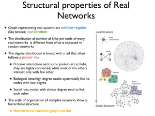
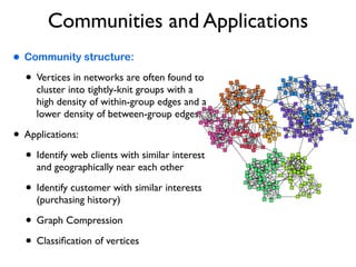
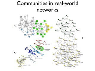
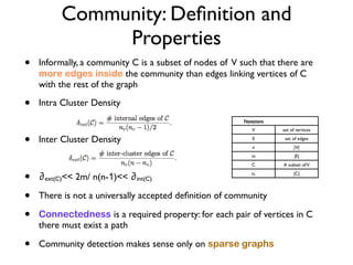
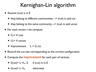
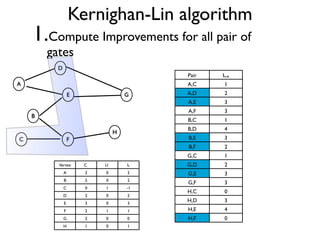
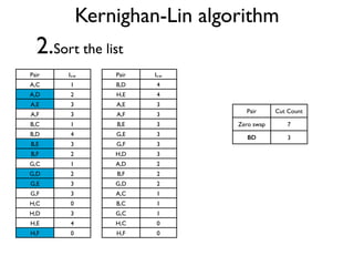
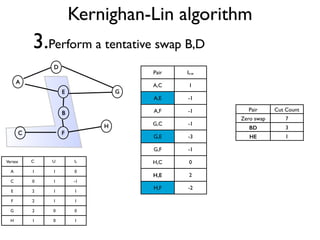
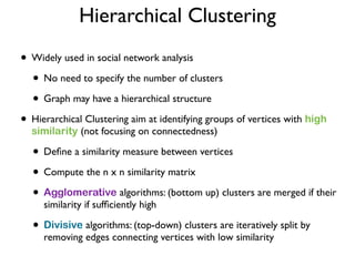
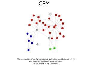
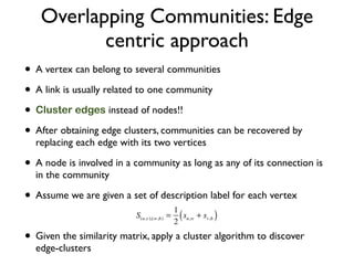
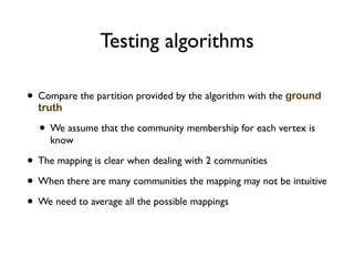
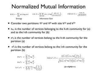
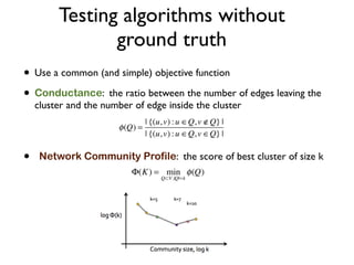
The document discusses community detection in graphs, highlighting how vertices in networks tend to cluster into groups with a high internal edge density. It covers various methods for detecting communities, such as the Kernighan-Lin algorithm, hierarchical clustering, and the Girvan-Newman method, while also addressing complexities like overlapping communities and the evaluation of detection algorithms. Additionally, it emphasizes the importance of modularity in assessing community structures and presents examples illustrating these concepts.

1. Community Detection
in Graphs
Nicola Barbieri
nicolabarbieri1@gmail.com
References:
Community Detection in Graphs, Santo Fortunato
Community Detection and Mining in Social Media, Lei Tang and Huan Liu

2. Zackary’s Karate Club
• Members of a university karate
club (unknown location)
• Zachary (1977) used these data to
explain the split-up of this group
following disputes among the
members.
• Conflict between the club
president, John A., and Mr. Hi over
the price of karate lessons
• The conflict results in "pulling"
apart the network of friendship
ties

3. Structural properties of Real
Networks
• Graph representing real systems are neither regular
(like lattices) nor random
• The distribution of number of links per node of many
real networks is different from what is expected in
random networks
• The degree distribution is broad, with a tail that often
follows a power law
• Proteins interaction nets: some protein act as hubs,
they are highly connected, while most of the others
interact only with few other
• Biological nets: high degree nodes systemically link to
nodes with low degree
• Social nets: nodes with similar degree tend to link
each other
• The scale of organization of complex networks show a
hierarchical structure
• Hierarchical random graph model

4. Communities and Applications
• Community structure:
• Vertices in networks are often found to
cluster into tightly-knit groups with a
high density of within-group edges and a
lower density of between-group edges.
• Applications:
• Identify web clients with similar interest
and geographically near each other
• Identify customer with similar interests
(purchasing history)
• Graph Compression
• Classification of vertices

5. Communities in real-world
networks

6. Relationships in real-world
networks
• Link direction
• Relationships between nodes may not to be reciprocal
• In the Web few hyperlinks are reciprocal (<10%)
• Community detection on directed graph is a hard task
• Overlapping Communities: some vertices may belong to more than one
group
• Heterogeneous Networks: different classes of vertices, playing different
roles
• Multipartite Networks
• Weighted relationships

7. Finding Communities
• Given a graph G=<V,E>
• Community detection problem: find modules and their
hierarchical organization
• What do we miss?
• Define what is “a community”
• Design algorithms that will find set of nodes which lead to “good
communities”
• Why just “good”??
• Evaluate different results

8. Community: Definition and
Properties
• Informally, a community C is a subset of nodes of V such that there are
more edges inside the community than edges linking vertices of C
with the rest of the graph
• Intra Cluster Density
• Inter Cluster Density
• ∂ext(C)<< 2m/ n(n-1)<< ∂int(C)
• There is not a universally accepted definition of community
• Connectedness is a required property: for each pair of vertices in C
there must exist a path
• Community detection makes sense only on sparse graphs
Notations
V set of vertices
E set of edges
n |V|
m |E|
C A subset ofV
nc |C|

9. Local Definitions
• Clique: subset of V such that all the vertices are adjacent to each
other
• Triangles are really frequent in real networks
• Finding cliques in a graph is NP Complete
• Too strict definition
• k-clique: is a maximal subgraph in which the largest geodesic
distance between any two nodes is no greater than k
• k-club: restricts the geodesic distance within the group to be no
greater than k

10. Global Definitions
• Communities can be also defined with respect to the whole graph
• A graph has a community structure if it is different from a random
graph
• A random graph is not expected to have any community structure:
• any two vertices have the same probability to be adjacent
• We can define a null model and use it to investigate whether the
graph under consideration exhibit a community structure

11. Similarity
• A community can be defined as a subset of vertices that are similar
to each other
• Do not consider connection
• Structural equivalence: v1 and v2 are structural equivalent if they
share the same neighbors and they are not adjacent
• Overlap between the neighborhoods Γ(i) and Γ(j) of vertices i and j
• Pearson
• Commute-time: average number of steps needed for a random
walker, starting at either vertex, to reach the other vertex for the first
time and to come back to the starting vertex

12. Partitions
• A partition is a division of a graph in clusters, such that each vertex belongs
to one cluster
• The Stirling numbers of the second kind count the number of ways to
partition a set of n labelled objects into k nonempty unlabelled subsets
• Hierarchical organization
• Communities embedded within other communities
• Nodes can be shared between different communities

13. Comparing Different partitions
• What is a good clustering?
• A quality function is a function that assigns a number to each
partition of a graph
• We can rank partitions based on their score given by the quality
function.
• A quality function Q is additive if there is an elementary function q
such that, for any partition P of a graph
• Performance P
• # vertices belonging to the same community
and connected by an edge
• # vertices belonging to different communities
and not connected by an edge.

14. Modularity
• The most popular quality function is the modularity
density of edges in a subgraph vs density
in a null model graph
• The δ-function yields one if vertices i and j are in the same
community, zero otherwise
• Pij represents the expected number of edges between vertices i and j
in the null model (which is arbitrary)
• Bernulli random graph
• Configuration model
ki = degree of the vertex (i)
• nc is the number of clusters,
• lc the total number of edges joining vertices of module c
• dc the sum of the degrees of the vertices of c.
a b
c
d
e
a
b
c
d
e

15. Graph Partitioning
• Divide the vertices in k groups of predefined size, such that the
number of edges lying between the groups is minimal
• The number of edges running between clusters is called cut size
• Specifying the number of clusters of the partition is necessary

16. Kernighan-Lin algorithm
• Heuristic procedure for the problem of partitioning electronic circuits onto
boards
• Iterative Improvement:
• Generate an initial solution
• Update the current solution iteratively, until we have an optimal solution
• KL-Algorithm O(n2 log n):
• An initial partition is generated at random
• A solution is acceptable if both the communities contain the same
number of vertices
• The cut size is the goodness of a solution
• Update: Select a subset of pair of vertices (u,v), where u belongs to C1
and v to C2 and swap them

17. Kernighan-Lin algorithm
• Assume (v,w) is in E
• they belong to different communities --> (v,w) is said cut
• they belong to the same community --> (v,w) is said uncut
• For each vertex v we compute
• Cv= # cuts
• Uv= # uncuts
• Improvement Iv = Cv-Uv
• Record the cut size corresponding to the current configuration
• Compute the improvement for each pair of vertices
• I(v,w)= Iv +Iw -2 if (v,w) is in E
• I(v,w)= Iv +Iw otherwise

18. Kernighan-Lin algorithm
1.Compute Improvements for all pair of
gates
A
B
D
C
E G
H
F
Vertex C U Iv
A 2 0 2
B 2 0 2
C 0 1 -1
D 2 0 2
E 3 0 3
F 2 1 1
G 2 0 0
H 1 0 1
Pair Iv.w
A,C 1
A,D 2
A,E 3
A,F 3
B,C 1
B,D 4
B,E 3
B,F 2
G,C 1
G,D 2
G,E 3
G,F 3
H,C 0
H,D 3
H,E 4
H,F 0

19. Kernighan-Lin algorithm
2.Sort the list
Pair Iv.w
A,C 1
A,D 2
A,E 3
A,F 3
B,C 1
B,D 4
B,E 3
B,F 2
G,C 1
G,D 2
G,E 3
G,F 3
H,C 0
H,D 3
H,E 4
H,F 0
Pair Iv.w
B,D 4
H,E 4
A,E 3
A,F 3
B,E 3
G,E 3
G,F 3
H,D 3
A,D 2
B,F 2
G,D 2
A,C 1
B,C 1
G,C 1
H,C 0
H,F 0
Pair Cut Count
Zero swap 7
BD 3

20. Kernighan-Lin algorithm
3.Perform a tentative swap B,D
Pair Iv.w
A,C 1
A,E -1
A,F -1
G,C -1
G,E -3
G,F -1
H,C 0
H,E 2
H,F -2
Vertex C U Iv
A 1 1 0
C 0 1 -1
E 2 1 1
F 2 1 1
G 2 0 0
H 1 0 1
A
B
D
C
E G
H
F
Pair Cut Count
Zero swap 7
BD 3
HE 1

21. Kernighan-Lin algorithm
2.Perform a tentative swap H,E
Pair Iv.w
A,C -3
A,F -5
G,C -3
G,F -5
Vertex C U Iv
A 0 2 -2
C 0 1 -1
F 0 3 -3
G 0 2 -2
A
B
D
C
E G
H
F
Pair Cut Count
Zero swap 7
BD 3
HE 1
AC 3

22. Kernighan-Lin algorithm
5.Perform a tentative swap A,C
Pair Iv.w
G,F -3
Vertex C U Iv
F 1 2 -1
G 0 2 -2
A B
D
C
E G
H
F
Pair Cut Count
Zero swap 7
BD 3
HE 1
AC 4
GF 7

23. Kernighan-Lin algorithm
6.Scan the list searching for the min cut
7.Perform the swaps (if the min cut < zero swaps)
Pair Cut Count
Zero swap 7
BD 3
HE 1
AC 4
GF 7
A
B
D
C
E G
H
F A
B
D
C
E G
H
F8. Second iteration

24. Hierarchical Clustering
• Widely used in social network analysis
• No need to specify the number of clusters
• Graph may have a hierarchical structure
• Hierarchical Clustering aim at identifying groups of vertices with high
similarity (not focusing on connectedness)
• Define a similarity measure between vertices
• Compute the n x n similarity matrix
• Agglomerative algorithms: (bottom up) clusters are merged if their
similarity if sufficiently high
• Divisive algorithms: (top-down) clusters are iteratively split by
removing edges connecting vertices with low similarity

25. Hierarchical Clustering
• Merging Clusters
• Single linkage
• Complete linkage
• Average linkage
• Drawback of the hierarchical procedure: it does not provide a way to
discriminate which level better represents the community structure
of the graph

26. Girvan-Newman
• Divisive method: detect edges that connect different communities and
remove them until clusters are disconnected
• 4 Steps:
1.Compute Edge centrality
2.Remove the edge with the highest centrality
3.Update (!!!!) Centralities
4.If |E|>0, go to 2

27. Girvan-Newman
• Instead of trying to construct a measure which tells us which edges are
most central to communities, we focus instead on those edges which are
least central
• If a network contains communities or groups that are only loosely
connected by a few inter-group edges, then all shortest paths between
different communities must go along one of these few edges
• Edge Betweenness O(mn)
• number of shortest path between all vertex
pair that run along the considered edge
• The edges connecting communities will have
high edge betweenness
• Which partition is the best???
• Compute modularity

28. Girvan-Newman
Optimal community structure for Zachary's karate club.
Modularity without recalculation

29. Modularity optimization
• If high modularity indicate goods partition, why not simply optimize Q
over all partitions to find the best one?
• The search-space is exponential in |V|
• Greedy algorithm (Newman):
• Agglomerative clustering: we repeatedly join communities together in
pairs, choosing at each step the join that results in the greatest increase
(or smallest decrease) in Q
• Note that the joining of a pair of communities between which there are
no edges at all can never result in an increase in Q.This limit the number
of tentative joins to (m)
eii is the fraction of edges in the network
that connect vertices in the group i
ai is the fraction of edges that connect
vertices in the group i with every other group

30. Modularity optimization
C1
C2
C3
C4
m=24

31. Modularity optimization
• The peak modularity is Q = 0.381
• The GN algorithm performs similarly on this task, but not better it
also finds the split but classifies one vertex wrongly (although a
different one, vertex 3).

32. Overlapping Communities
• The most popular technique to discover
overlapping communities is the Clique
Percolation Method (CPM)
• The internal edges of a community are likely
to form cliques due to their high density
• It is unlikely that inter-community edges form
cliques
• If it were possible for a clique to move on a
graph, in some way, it would probably get
trapped inside its original community, as it
could not cross the bottleneck formed by the
inter-community edges

33. CPM
• Given a parameter k:
1.Find all the cliques of size k
2.Construct a clique graph. 2 cliques are adjacent if they share k-1
vertices
3.Each connect component of the clique graph is a community
cliques of size 3= {1,2,3}, {1,3,4},{4,5,6},{5,6,7},
{5,6,8},{5,7,8},{6,7,8}
{1,2,3}
{1,3,4}
{4,5,6}
{5,6,7}
{5,6,8}
{5,7,8} {6,7,8}

34. CPM
The communities of the Karate network (by k-clique percolation for k = 3):
gray nodes are overlapping and white nodes
do not belong to any community

35. Overlapping Communities: Edge
centric approach
• A vertex can belong to several communities
• A link is usually related to one community
• Cluster edges instead of nodes!!
• After obtaining edge clusters, communities can be recovered by
replacing each edge with its two vertices
• A node is involved in a community as long as any of its connection is
in the community
• Assume we are given a set of description label for each vertex
• Given the similarity matrix, apply a cluster algorithm to discover
edge-clusters

36. Testing algorithms
• Compare the partition provided by the algorithm with the ground
truth
• We assume that the community membership for each vertex is
know
• The mapping is clear when dealing with 2 communities
• When there are many communities the mapping may not be intuitive
• We need to average all the possible mappings

37. Normalized Mutual Information
• Consider two partitions πa and πb with size k(a) and k(b)
• nh,l is the number of vertices belonging to the h-th community for (a)
and to the l-th community for (b)
• na
h is the number of vertices belong to the h-th community for the
partition (a)
• nb
l is the number of vertices belong to the l-th community for the
partition (b)
Entropy Information Gain
0<=NMI<=1

38. Testing algorithms without
ground truth
• Use a common (and simple) objective function
• Conductance: the ratio between the number of edges leaving the
cluster and the number of edge inside the cluster
• Network Community Profile: the score of best cluster of size k