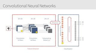
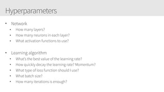
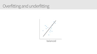
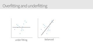
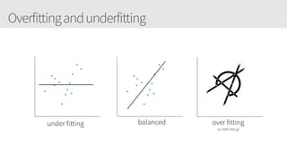
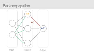
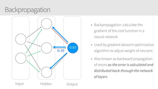
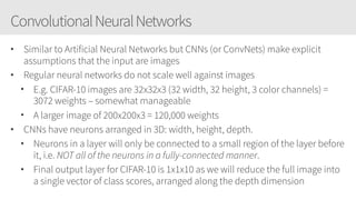
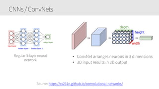
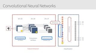
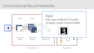
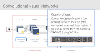
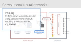
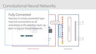
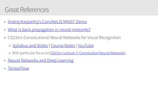
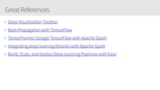
The document outlines a training series on neural networks focused on concepts and practical applications using Keras. It covers tuning, optimization, and training algorithms, alongside challenges such as overfitting and underfitting, and discusses the architecture and advantages of convolutional neural networks (CNNs). The content is designed for individuals interested in understanding deep learning fundamentals and applying them effectively.

1. Training Neural Networks

2. Accelerate innovation by unifying data science, engineering
and business
• Founded by the original creators of Apache Spark
• Contributes 75% of the open source code, 10x more than
any other company
• Trained 100k+ Spark users on the Databricks platform
VISION
WHO WE ARE
Unified Analytics Platform powered by Apache Spark™PRODUCT

3. Aboutourspeaker
Denny Lee
Technical Product Marketing Manager
Former:
• Senior Director of Data Sciences Engineering at SAP Concur
• Principal Program Manager at Microsoft
• Azure Cosmos DB Engineering Spark and Graph Initiatives
• Isotope Incubation Team (currently known as HDInsight)
• Bing’s Audience Insights Team
• Yahoo!’s 24TB Analysis Services cube

4. DeepLearningFundamentalsSeries
This is a three-part series:
• Introduction to Neural Networks
• Training Neural Networks
• Applying your Convolutional Neural Network
This series will be make use of Keras (TensorFlow backend) but as it is a
fundamentals series, we are focusing primarily on the concepts.

5. PreviousSession:IntroductiontoNeuralNetworks
• What is Deep Learning?
• What can Deep Learning do for you?
• What are artificial neural networks?
• Let’s start with a perceptron…
• Understanding the effect of activation functions

6. CurrentSession:TrainingNeuralNetworks
• Tuning training
• Training Algorithms
• Optimization (including Adam)
• Convolutional Neural Networks

7. UpcomingSession:ApplyingNeuralNetworks
• Diving further into CNNs
• CNN Architectures
• Convolutions at Work!

8. Convolutional Neural Networks
28 x 28 28 x 28 14 x 14
Convolution
32 filters
Convolution
64 filters
Subsampling
Stride (2,2)
Feature Extraction Classification
0
1
8
9
FullyConnected
Dropout
Dropout

9. Tuning Training

10. Hyperparameters
• Network
• How many layers?
• How many neurons in each layer?
• What activation functions to use?
• Learning algorithm
• What’s the best value of the learning rate?
• How quickly decay the learning rate? Momentum?
• What type of loss function should I use?
• What batch size?
• How many iterations is enough?

11. Overfittingandunderfitting

12. Overfittingandunderfitting

13. Overfittingandunderfitting

14. Hyperparameters:Network
Generally, the more layers and the number of units in each layer:
• The greater the capacity of the artificial neural network
• The risk is overfitting when your goal is to build a generalized model.
From a practical perspective, a good starting point is:
• The number of input units equals the dimension of features
• The number of output units equals the number of classes (e.g. in the MNIST dataset, there
are 10 possible values represents digits (0…9) hence there are 10 output units
• Start with one hidden layer that is 2x the number of input units
• A good reference is Andrew Ng’s Coursera Machine Learning course.

15. Hyperparameters:ActivationFunctions?
• Good starting point: ReLU
• Note many neural networks samples: Keras MNIST, TensorFlow CIFAR10 Pruning, etc.
• Note that each activation function has its own strengths and weaknesses. A good quote
on activation functions from CS231N summarizes the choice well:
“What neuron type should I use?” Use the ReLU non-linearity, be careful with your learning rates
and possibly monitor the fraction of “dead” units in a network. If this concerns you, give Leaky
ReLU or Maxout a try. Never use sigmoid. Try tanh, but expect it to work worse than ReLU/
Maxout.

16. Neurons … Activate!
DEMO

17. Hyperparameters
Learning algorithm
• What’s the best value of the learning rate?
• How quickly decay the learning rate? Momentum?
• What type of loss function should I use?
• What batch size?
• How many iterations is enough?

18. Training Algorithms

19. Cost function
Source: https://bit.ly/2IoAGzL
For this linear regression example, to
determine the best (slope of the line) for
we can calculate the cost function, such as
Mean Square Error, Mean absolute error,
Mean bias error, SVM Loss, etc.
For this example, we’ll use sum of squared
absolute differences
𝑦 = 𝑥 ⋅ 𝑝
𝑝
𝑐𝑜𝑠𝑡 =
∑
| 𝑡 − 𝑦|2

20. Gradient Descent Optimization
Source: https://bit.ly/2IoAGzL

21. Small Learning Rate
Source: https://bit.ly/2IoAGzL

22. Small Learning Rate
Source: https://bit.ly/2IoAGzL

23. Small Learning Rate
Source: https://bit.ly/2IoAGzL

24. Small Learning Rate
Source: https://bit.ly/2IoAGzL

25. SimplifiedTwo-LayerANN
1
1
0.8
0.2
0.7
0.6
0.9
0.1
0.8
0.75
0.69
h1 = 𝜎(1𝑥0.8 + 1𝑥0.6) = 0.80
h2 = 𝜎(1𝑥0.2 + 1𝑥0.9) = 0.75
h3 = 𝜎(1𝑥0.7 + 1𝑥0.1) = 0.69

26. SimplifiedTwo-LayerANN
1
1
0.8
0.2
0.7
0.6
0.9
0.1
0.8
0.75
0.69
0.2
0.8
0.5
0.75
𝑜𝑢𝑡 = 𝜎(0.2𝑥0.8 + 0.8𝑥0.75 + 0.5𝑥0.69)
= 𝜎(1.105)
= 0.75

27. Backpropagation
Input Hidden Output
0.8
0.2
0.75

28. Backpropagation
Input Hidden Output
0.85
• Backpropagation: calculate the
gradient of the cost function in a
neural network
• Used by gradient descent optimization
algorithm to adjust weight of neurons
• Also known as backward propagation
of errors as the error is calculated and
distributed back through the network
of layers
0.10

29. Sigmoidfunction(continued)
Output is not zero-centered: During gradient
descent, if all values are positive then during
backpropagation the weights will become all
positive or all negative creating zig zagging
dynamics.
Source: https://bit.ly/2IoAGzL

30. LearningRateCallouts
• Too small, it may take too long to get minima
• Too large, it may skip the minima altogether

31. Optimization

32. OptimizationOverview
• After backpropagation, the parameters are updated based on the gradients
calculated
• There are several approaches in this area of active research; we will focus on:
• Stochastic Gradient Descent
• Momentum, NAG
• Per-parameter adaptive learning rate methods

33. StochasticGradientDescent
• (Batch) Gradient Descent is computed on the full dataset (not efficient for large
scale models and datasets).
• Often converges faster because it performs updates more frequently
• But due to frequent updates, this may complicate convergence to the exact
minima
• For more information, refer to:
• Andrew Ng’s 2. Stochastic Gradient (https://goo.gl/bNrJbx)
• Types of Optimization Algorithms used in Neural Networks and Ways to
Optimize Gradient Descent (https://goo.gl/tB2e7S)

34. GradientDescent Source: https://goo.gl/VUX2ZS

35. MomentumandNAG
• Obtain faster convergence by helping parameter vector build up velocity
• i.e. use the momentum of the gradient to converge faster
• Nesterov Accelerated Gradient (NAG): optimized version of Momentum
• Typically works better in practice than Momentum
Source: http://cs231n.github.io/neural-networks-3

36. Annealingthelearningrate
• i.e. slow down the learning rate to prevent it from bouncing around too much
• Referred as the decay parameter (i.e., the learning rate decay over each
update) to reduce kinetic energy
• Note, this is different from rho (i.e. exponentially weighted average or
exponentially weighted decay of past gradients) to smooth the descent path
trajectory

37. Per-parameteradaptivelearningratemethods
• Adaptively tune learning rates at the parameter level
• Popular methods include:
• Adaptive Gradient Algorithm (AdaGrad) improves performance on problems with sparse
gradients (e.g. natural language and computer vision problems).
• Root Mean Square Propagation (RMSProp) maintains per-parameter learning rates based
on the average of recent magnitudes of the gradients for the weight (e.g. how quickly it is
changing). This means the algorithm does well on online and non-stationary problems
(e.g. noisy).
• AdaDelta: Per dimension learning rate method for gradient descent with minimal
computational overhead, requires no manual tuning, and quite robust

38. WhichOptimizer?
“In practice Adam is currently recommended as
the default algorithm to use, and often works
slightly better than RMSProp. However, it is often
also worth trying SGD+Nesterov Momentum as
an alternative..”
Andrej Karpathy, et al, CS231n
Source: https://goo.gl/2da4WY
Comparison of Adam to Other Optimization Algorithms Training a Multilayer Perceptron
Taken from Adam: A Method for Stochastic Optimization, 2015.

39. Optimizationonlosssurfacecontours
Adaptive algorithms converge
quickly and find the right direction
for the parameters.
In comparison, SGD is slow
Momentum-based methods
overshoot
Source: http://cs231n.github.io/neural-networks-3/#hyper
Image credit: Alec Radford

40. Optimizationonsaddlepoint
Notice how SGD gets stuck near the
top
Meanwhile adaptive techniques
optimize the fastest
Source: http://cs231n.github.io/neural-networks-3/#hyper
Image credit: Alec Radford

41. GoodReferences
• Suki Lau's Learning Rate Schedules and Adaptive Learning Rate Methods for
Deep Learning
• CS23n Convolutional Neural Networks for Visual Recognition
• Fundamentals of Deep Learning
• ADADELTA: An Adaptive Learning Rate Method
• Gentle Introduction to the Adam Optimization Algorithm for Deep Learning

42. Convolutional Networks

43. ConvolutionalNeuralNetworks
• Similar to Artificial Neural Networks but CNNs (or ConvNets) make explicit
assumptions that the input are images
• Regular neural networks do not scale well against images
• E.g. CIFAR-10 images are 32x32x3 (32 width, 32 height, 3 color channels) =
3072 weights – somewhat manageable
• A larger image of 200x200x3 = 120,000 weights
• CNNs have neurons arranged in 3D: width, height, depth.
• Neurons in a layer will only be connected to a small region of the layer before
it, i.e. NOT all of the neurons in a fully-connected manner.
• Final output layer for CIFAR-10 is 1x1x10 as we will reduce the full image into
a single vector of class scores, arranged along the depth dimension

44. CNNs/ConvNets
Regular 3-layer neural
network
• ConvNet arranges neurons in 3 dimensions
• 3D input results in 3D output
Source: https://cs231n.github.io/convolutional-networks/

45. Convolutional Neural Networks
28 x 28 28 x 28 14 x 14
Convolution
32 filters
Convolution
64 filters
Subsampling
Stride (2,2)
Feature Extraction Classification
0
1
8
9
FullyConnected
Dropout
Dropout

46. Convolutional Neural Networks
28 x 28 28 x 28 14 x 14
Convolution
32 filters
Convolution
64 filters
Subsampling
Stride (2,2)
Feature Extraction Classification
0
1
8
9
FullyConnected
Dropout
Dropout
Input
Pixel value of 32x32x3: 32 width,
32 height, 3 color channels (RGB)

47. Convolutional Neural Networks
28 x 28 28 x 28 14 x 14
Convolution
32 filters
Convolution
64 filters
Subsampling
Stride (2,2)
Feature Extraction Classification
0
1
8
9
FullyConnected
Dropout
Dropout
Convolutions
Compute output of neurons (dot
product between their weights)
connected to a small local region. If
we use 32 filters, then the output is
28x28x32 (using 5x5 filter)

48. Convolutional Neural Networks
28 x 28 28 x 28 14 x 14
Convolution
32 filters
Convolution
64 filters
Subsampling
Stride (2,2)
Feature Extraction Classification
0
1
8
9
FullyConnected
Dropout
Dropout
Pooling
Perform down sampling operation
along spatial dimensions (w, h)
resulting in reduced volume,
e.g. 14x14x2.

49. Convolutional Neural Networks
28 x 28 28 x 28 14 x 14
Convolution
32 filters
Convolution
64 filters
Subsampling
Stride (2,2)
Feature Extraction Classification
0
1
8
9
FullyConnected
Dropout
Dropout
Fully Connected
Neurons in a fully connected layer
have full connections to all
activations in the previous layer, as
seen in regular Neural Networks.

50. https://cs.stanford.edu/people/karpathy/convnetjs/demo/mnist.html
ConvNetJS MNIST Demo

51. Neurons … Activate!
DEMO

52. I’d like to thank…

53. GreatReferences
• Andrej Karparthy’s ConvNetJS MNIST Demo
• What is back propagation in neural networks?
• CS231n: Convolutional Neural Networks for Visual Recognition
• Syllabus and Slides | Course Notes | YouTube
• With particular focus on CS231n: Lecture 7: Convolution Neural Networks
• Neural Networks and Deep Learning
• TensorFlow

54. GreatReferences
• Deep Visualization Toolbox
• Back Propagation with TensorFlow
• TensorFrames: Google TensorFlow with Apache Spark
• Integrating deep learning libraries with Apache Spark
• Build, Scale, and Deploy Deep Learning Pipelines with Ease

55. Attribution
Tomek Drabas
Brooke Wenig
Timothee Hunter
Cyrielle Simeone

56. Q&A

57. What’s next?
Applying your Convolutional Neural Network
October 25, 2018 | 10:00 PDT
https://dbricks.co/2O2c4BZ
State Of The Art Deep Learning On Apache Spark™
October 31, 2018 | 09:00 PDT
https://dbricks.co/2NqogIp