Download as PDF, PPTX


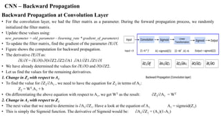
![CNN – Backward Propagation
• CNN contains three parameters – weights, biases and filters. Let calculate the gradients for these parameters one by one.
Backward Propagation at Fully Connected Layer
• Fully connected layer has two parameters – weight matrix and bias matrix.
• Let us start by calculating the change in error with respect to weights – ∂E/∂W.
• Since the error is not directly dependent on the weight matrix, we will use the concept of chain rule to find this value.
• The computation graph shown below will help us define ∂E/∂W:
• ∂E/∂W = ∂E/∂O . ∂O/∂Z2. ∂z/∂W
Find these derivatives separately:
1. Change in error with respect to output
• Suppose the actual values for the data are denoted as y’ and
• the predicted output is represented as O.
• Then the error is: E = (y' - O)2/2
• If we differentiate the error with respect to the output: ∂E/∂O = -(y'-O)
2. Change in output with respect to Z2 (linear transformation output)
• To find the derivative of output O with respect to Z2, we must first define O in terms of Z2. The output is sigmoid of Z2.
Thus, ∂O/∂Z2 is effectively the derivative of Sigmoid function: f(x) = 1/(1+e^-x)
• The derivative of this function: f'(x) = (1+e-x)-1[1-(1+e-x)-1]
f'(x) = sigmoid(x)(1-sigmoid(x))
∂O/∂Z2 = (O)(1-O)](https://image.slidesharecdn.com/deeplearning-210816173438/85/Deep-learning-47-320.jpg)


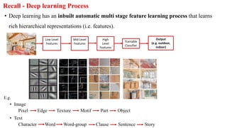


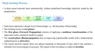
The document provides a detailed overview of deep learning, explaining the structure and functioning of artificial neural networks that mimic human brain operations. It discusses various components such as activation functions, training processes including forward and backward propagation, and the importance of hyper-parameters like learning rates and biases. Additionally, it covers applications of deep learning and different types of neural networks, emphasizing the benefits of deep learning over traditional machine learning methods.