Download as PDF, PPTX


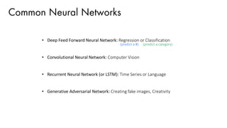
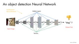
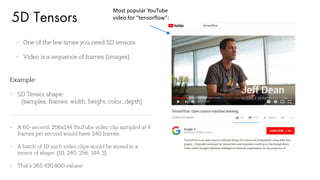
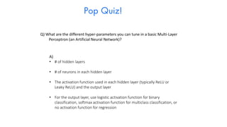
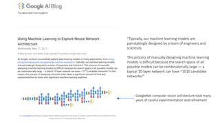
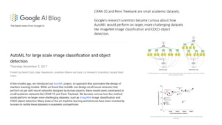
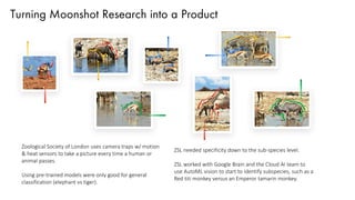
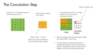
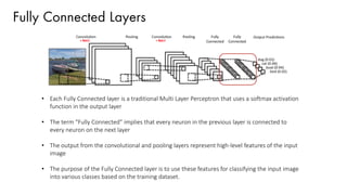
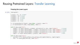
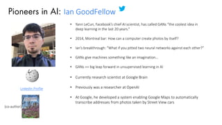
![Activation Functions
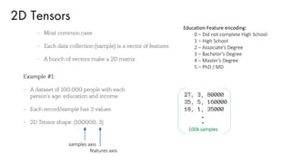
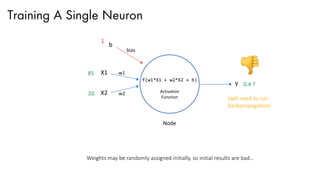
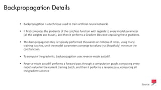
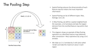
Sigmoid tanh ReLU Others
- takes a real-valued input
and squashes it to range
between 0 and 1
- takes a real-valued input
and squashes it to the
range [-1, 1]
- ReLU stands for Rectified
Linear Unit. It takes a
real-valued input and
thresholds it at zero
(replaces negative values
with zero)
LeakyReLU:
ELU:
Source:
2016 ELU Paper](https://image.slidesharecdn.com/3sameerfarooqui-180614202407/85/Separating-Hype-from-Reality-in-Deep-Learning-with-Sameer-Farooqui-23-320.jpg)

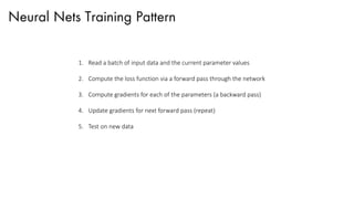

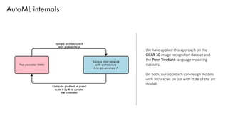
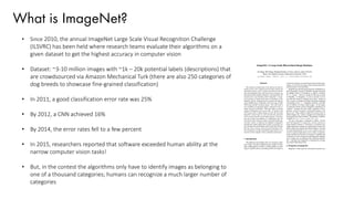

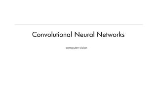
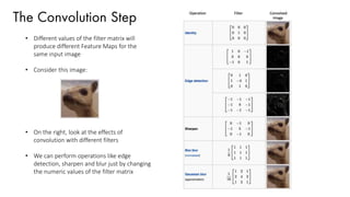
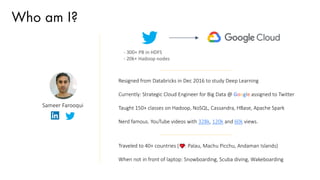
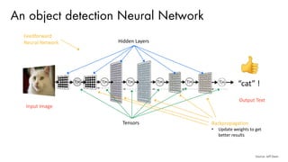
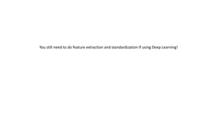
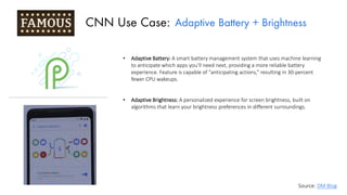
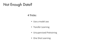
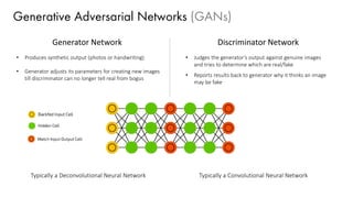
![Training using Backpropagation
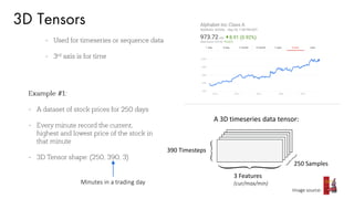
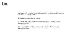
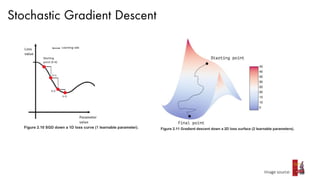
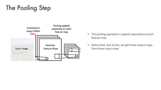
• Since the input image is a boat, the target probability is 1 for Boat class and 0 for other three classes, i.e.
• Input Image = Boat
• Target Vector = [0, 0, 1, 0]
• Use Backpropagation to calculate the gradients of the error with respect to all weights in the network and
use gradient descent to update all filter values / weights and parameter values to minimize the output error.](https://image.slidesharecdn.com/3sameerfarooqui-180614202407/85/Separating-Hype-from-Reality-in-Deep-Learning-with-Sameer-Farooqui-71-320.jpg)

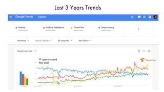
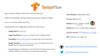
The document discusses deep learning trends and technologies, highlighting TensorFlow as a significant open-source machine learning library developed by Google for training neural networks. It also covers various neural network architectures and training methodologies, including convolutional neural networks (CNNs), recurrent neural networks (RNNs), and the use of AutoML for hyperparameter tuning and automated model design. Additionally, notable figures in AI like Geoffrey Hinton and Yann LeCun are mentioned along with advancements in computer vision applications.


![제 23회 보아즈(BOAZ) 빅데이터 컨퍼런스 - [MBOAX] : ABSA를 활용한 소비자 반응 분석 기반 운영 효율화 대시보드 설계](https://cdn.slidesharecdn.com/ss_thumbnails/3-1boaz23rdconferencemboax-260203102709-9d519923-thumbnail.jpg?width=640&height=640&fit=bounds)


