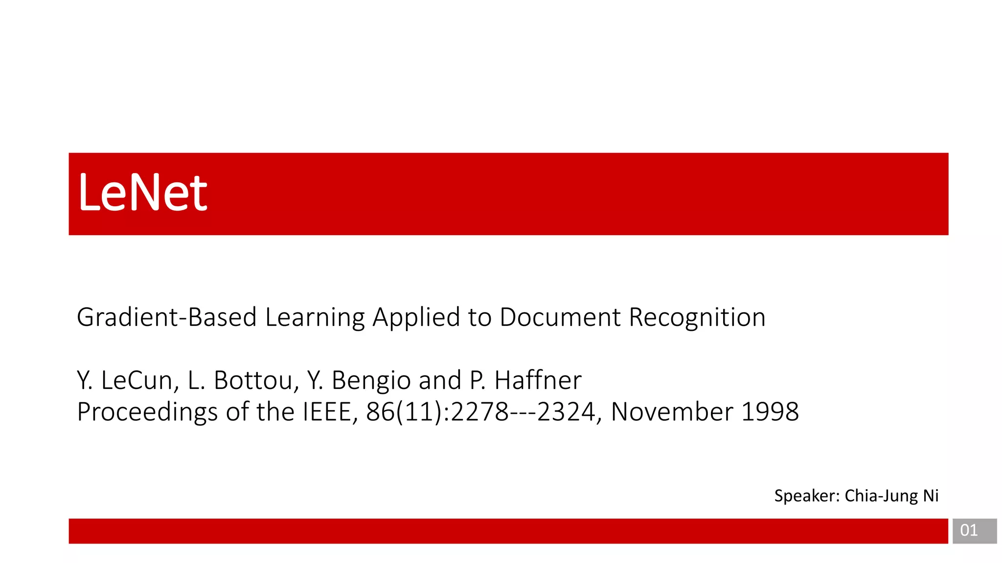
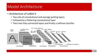
This document discusses the application of gradient-based learning for document recognition, focusing on Convolutional Neural Networks (CNNs) such as LeNet. Key concepts are introduced, including local receptive fields, shared weights, and sub-sampling, which contribute to the architecture's efficiency. The document also details the structure of the LeNet-5 model, its layers, and parameters involved in training and implementation.
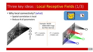
![11
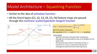
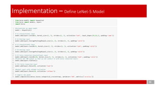
Model Architecture – 3rd layer (3/7)
• Trainable params
= ∑group [ (weight * input map channel + bias) * output map channel ]
= (5*5*3 + 1) * 6 + (5*5*4 + 1) * 6 + (5*5*4 + 1) * 3 + (5*5*6 + 1) * 1 = 456 + 606 + 303 +151 = 1,516
• Connections
= (weight * input map channel + bias) * output map channel * output map size
= [(5*5*3 + 1) * 6 + (5*5*4 + 1) * 6 + (5*5*4 + 1) * 3 + (5*5*6 + 1) * 1] * (10*10) = 151,600
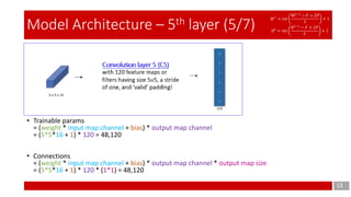
Convolution layer 3 (C3)
with 16 feature maps having
size 5×5 and a stride of one,
and ‘valid’ padding!
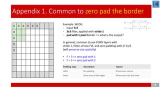
Based on the consideration of computation costs,
• First 6 feature maps are connected to 3 contiguous input maps
• Second 6 feature maps are connected to 4 contiguous input maps
• Next 3 feature maps are connected to 4 discontinuous input maps
• Last 1 feature map are connected to all 6 input maps
𝑊 𝑙
= 𝑖𝑛𝑡
W𝑙−1
− 𝐹 + 2𝑃
𝑆
+ 1
𝐻 𝑙
= 𝑖𝑛𝑡
𝐻 𝑙−1
− 𝐹 + 2𝑃
𝑆
+ 1](https://image.slidesharecdn.com/lenet-5-190622140937/85/LeNet-5-11-320.jpg)


![Polymer [ बहुलक ] Chemistry Notes PDF - Irfanullah Mehar - JJ Sir Chemistry.pdf](https://cdn.slidesharecdn.com/ss_thumbnails/polymerchemistrynotespdf-irfanullahmehar-jjsirchemistry-260210172118-3f9b37f7-thumbnail.jpg?width=640&height=640&fit=bounds)


