mann whitney u test

1. Mann-Whitney U-Test
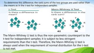
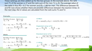
The Mann-Whitney U-Test can be
used to test whether there is a
difference between two groups,
and the data need not be normally
distributed.

2. To determine this difference, the rank sums of the two groups are used rather than
the means as in the t-test for independent samples.
The Mann-Whitney U test is thus the non-parametric counterpart to the
t-test for independent samples; it is subject to less stringent
requirements than the t-test. Therefore, the Mann-Whitney U test is
always used when the requirement of normal distribution for the t-test
is not met.

3. Assumptions Mann-Whitney U Tests
To be able to calculate a Mann-Whitney U test, only two independent
random samples with at least ordinally scaled characteristics must be
available. The variables do not have to satisfy any distribution curve.
If the data are available in pairs, the Wilcoxon test must be used instead of
the Mann-Whitney U test.

4. Hypotheses Mann-Whitney U-Tests
The hypotheses of the Mann-Whitney U-test are very similar to the
hypotheses of the independent t-test. The difference, however, is
that in the case of the Mann-Whitney U test, the test is based on a
difference in the central tendency, whereas in the case of the t test,
the test is based on a difference in the mean values. Thus, the
Mann-Whitney U test results in:
Null hypothesis: There is no difference (in terms of central
tendency) between the two groups in the population.
Alternative hypothesis: There is a difference (with respect to the
central tendency) between the two groups in the population.

5. Calculate Mann-Whitney U Test
To calculate the Mann-Whitney U test for two independent samples, the
rankings of the individual values must first be determined (An example with tied
ranks follows below).

6. These rankings are then added up for the two groups. In the example above, the rank
sum T1 of the women is 37 and the rank sum of the men T2 is 29. The average value of
the ranks is thus R̄1= 6.17 for women and R̄1= 5.80 for men. The difference between R̄1
and R̄2 now shows whether there are possible differences between the reaction times. In
the next step, the U-values are calculated from the rank sums T1 and T2.

7. where n1, n2 are the number of elements in the first and second group
respectively. If both groups are from the same population, i.e., the
groups do not differ, then the value of both U values is the expected
value of U. After the mean and dispersion have been estimated, z can
be calculated. For the Mann-Whitney U value, the smaller value of U1
and U2 is used.
Depending on how large the sample is, the p-value for the Mann-
Whitney U-test is calculated in a different way. For up to 25 cases, the
exact values are used, which can be read from a table. For larger
samples, the normal distribution can be used as an approximation. So,
in the present example one would actually take the exact value, here
nevertheless the way over the normal distribution. For this, the z-value
simply needs to be introduced into the z-value to p-value calculator

8. If the calculated z-value is larger than the critical z-value, the two
groups differ.

9. Calculate Mann-Whitney U test with tied ranks
If several people share a rank, connected ranks are present. In this case, there is a change in the
calculation of the rank sums and the standard deviation of the U-value. We will now go
through both using an example.
In the example it can be seen that the...
...reaction times 34 occur twice and share the ranks 2 and 3
...reaction times 39 occur three times and share the ranks 6, 7 and 8.

10. To account for these connected ranks, the mean values of the joined ranks are calculated in each
case. In the first case, this results in a "new" rank of 2.5 and in the second case in a "new" rank of
7. Now the rank sums T can be calculated.
Since the rank ties are clearly visible in the upper table, a term is calculated here that is needed
for the later calculation of the u-value in the presence of rank ties.
Now all values are available to calculate the z-value considering connected ranks.

11. Now all values are available to calculate the z-value considering connected ranks.

12. Again, noting that you actually need about 20 cases to assume normal distribution of u values.
Example with DATAtab
A Mann-Whitney U Test can be easily calculated with DATAtab. Simply copy the
table below or your own data into the statistics calculator and click on t-Test |
Chi2 Test | ANOVA | ... Then click on the two variables and select Non-Parametric
Test.
Reaction time women Reaction time men
34 45
36 33
41 35
43 39
44 42
29 39
44 43
37

13. DATAtab then gives you the following table for the Mann-Whitney U Test:
Mann-Whitney U Test Example
The Mann-Whitney-U-Test works with ranks, so the result will
first show the middle ranks and the rank sum. The reaction time
of women has a slightly lower value than that of men.

15. DATAtab gives you the asymptotic significance and the exact significance. The significance used depends on the sample
size. As a rule:
n1 + n2 < 30 -> exact significance
n1 + n2 > 30 -> asymptotic significance
Therefore the exact significance is used for this example. The significance (2-tailed) is 0.867 and thus above the
significance level of 0.05. Therefore, no difference between the reaction time of men and women can be determined
with these data.
Interpret Mann-Whitney-U-Test
The reaction time female group had the same high values (Mdn= 39) as the reaction time male group (Mdn= 39). A
Mann-Whitney U-Test showed that this difference was not statistically significant, U=26.5, p=.862, r=.045.
Mann-Whitney-U-Test Effect Size
In order to make a statement about the Effect Size in the Mann-Whitney-U-Test, you need the Standardised test statistic
z and the number of pairs n, with this you can then calculate the Effect Size with the formula below
Mann-Whitney U Test Effect size
In this case, an Effect Size r of 0.012. In general, one can say about the effect strength:
Effect Size r less than 0.3 -> small effect
Effect Size r between 0.3 and 0.5 -> medium effect
Effect Size r greater than 0.5 -> large effect
In this case, the Effect Size of 0.012 is therefore a small effect.