Here full information about Non Parametric Tests used in Statistics

1. B Y
P R O F . R A J E E V P A N D E Y
D E P A R T M E N T O F S T A T I S T I C S
U N I V E R S I T Y O F L U C K N O W
L U C K N O W
LECTURE
on
Parametric and Non-Parametric Tests
Chi-Square test, ANOVA, Mann-Whitney,
Kruskal Wallis and Kolmogrov-Smirnov

2. Nonparametrics and
goodness of fit
 In tests we have done so far, the null hypothesis
has always been a stochastic model with a few
parameters.
 T tests
 Tests for regression coefficients
 Test for autocorrelation
 …
 In nonparametric tests, the null hypothesis is not a
parametric distribution, rather a much larger class
of possible distributions

3. Nonparametric statistics
 The null hypothesis is for example that the
median of the distribution is zero
 A test statistic can be formulated, so that
it has a known distribution under this
hypothesis
it has more extreme values under
alternative hypotheses

4. Nonparametric tests: features
 Nonparametric statistical tests can be used when the data
being analysed is not a normal distribution
 Many nonparametric methods do not use the raw data and
instead use the rank order of data for analysis
 Nonparametric methods can be used with small samples

5. The sign test
 Assume the null hypothesis is that the
median of the distribution is zero.
 Given a sample from the distribution, there
should be roughly the same number of
positive and negative values.
 More precisely, number of positive values
should follow a binomial distribution with
probability 0.5.
 When the sample is large, the binomial
distribution can be approximated with a
normal distribution

6. Using the sign test: Example
 Patients are asked to value doctors they have visited
on a scale from 1 to 10.
 78 patiens have both visitied doctors A and B, and we
would like to find out if patients generally like one of
them better than the other. How?

7. Wilcoxon signed rank test
 Here, the null hypothesis is a symmetric
distribution with zero median. Do as follows:
 Rank all values by their absolute values.
 Let T+ be the sum of ranks of the positive values, and T-
corresponding for negative values
 Let T be the minimum of T+ and T-
 Under the null hypothesis, T has a known distribution.
 For large samples, the distribution can be
approximated with a normal distribution

8. Examples
 Often used on paired data.
 We want to compare primary health care costs for the
patient in two countries: A number of people having lived
in both countries are asked about the difference in costs per
year. Use this data in test.
 In the previous example, if we assume all patients attach
the same meaning to the valuations, we could use Wilcoxon
signed rank test on the differences in valuations

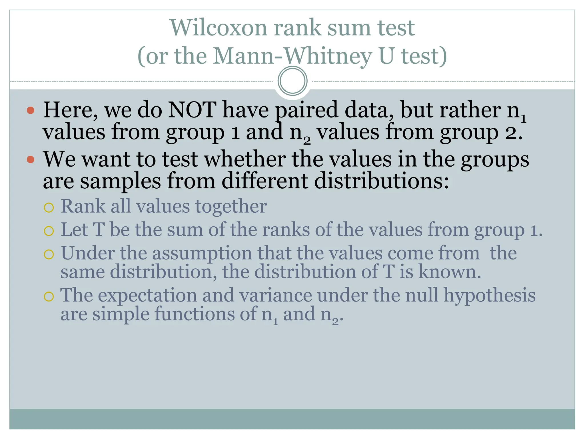
9. Wilcoxon rank sum test
(or the Mann-Whitney U test)
 Here, we do NOT have paired data, but rather n1
values from group 1 and n2 values from group 2.
 We want to test whether the values in the groups
are samples from different distributions:
 Rank all values together
 Let T be the sum of the ranks of the values from group 1.
 Under the assumption that the values come from the
same distribution, the distribution of T is known.
 The expectation and variance under the null hypothesis
are simple functions of n1 and n2.

10. Wilcoxon rank sum test
(or the Mann-Whitney U test)
 For large samples, we can use a normal
approximation for the distribution of T.
 The Mann-Whitney U test gives exactly the same
results, but uses slightly different test statistic.

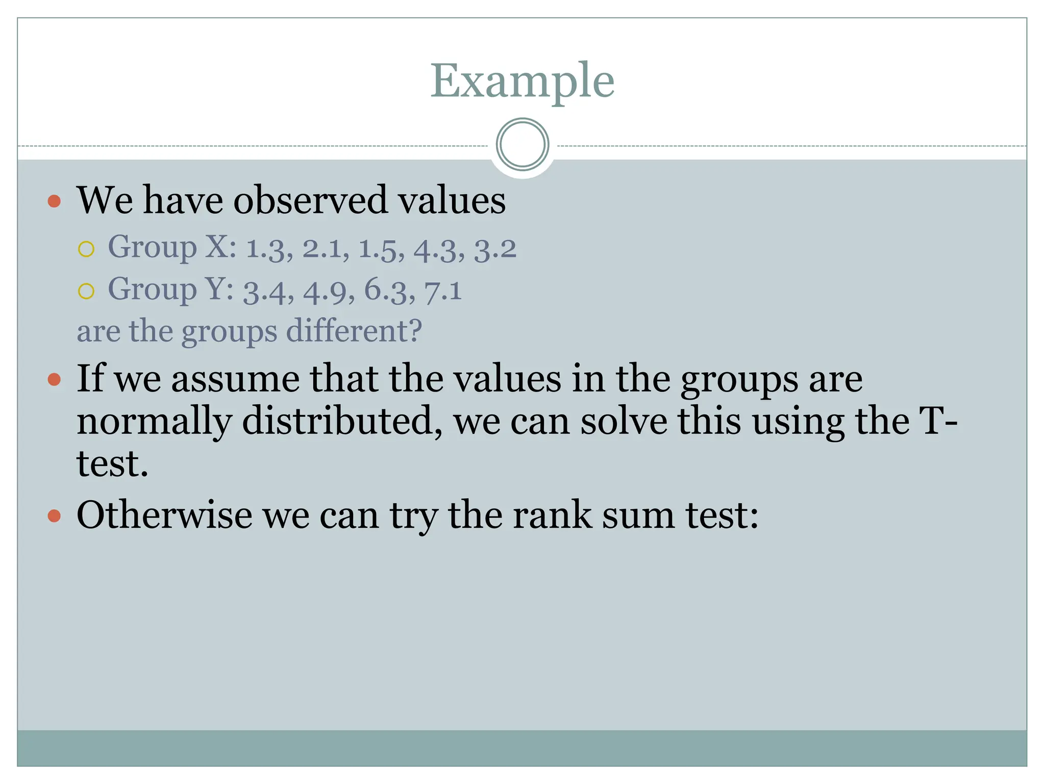
11. Example
 We have observed values
 Group X: 1.3, 2.1, 1.5, 4.3, 3.2
 Group Y: 3.4, 4.9, 6.3, 7.1
are the groups different?
 If we assume that the values in the groups are
normally distributed, we can solve this using the T-
test.
 Otherwise we can try the rank sum test:

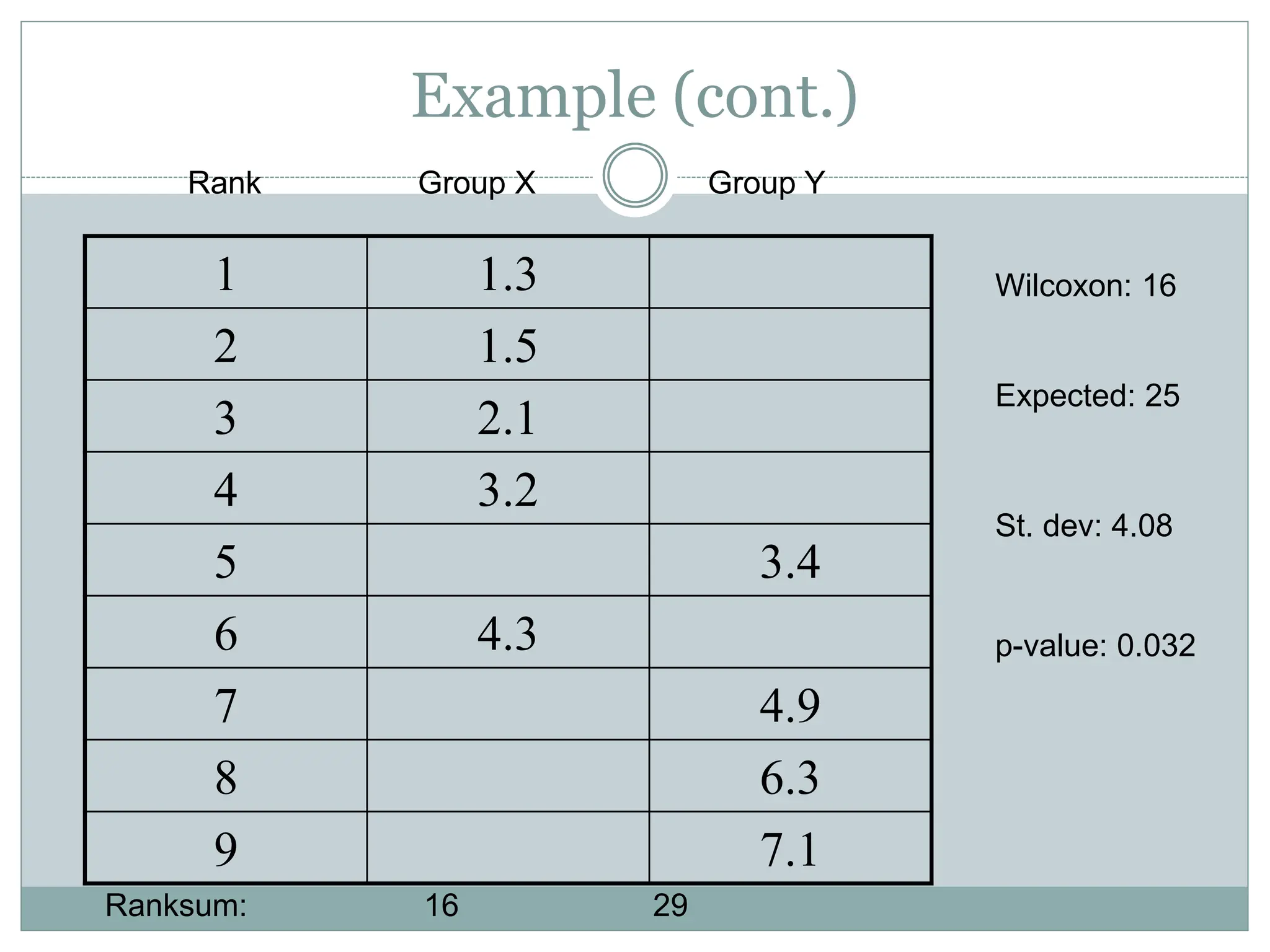
12. Example (cont.)
1 1.3
2 1.5
3 2.1
4 3.2
5 3.4
6 4.3
7 4.9
8 6.3
9 7.1
Rank Group X Group Y
Ranksum: 16 29
Wilcoxon: 16
Expected: 25
St. dev: 4.08
p-value: 0.032

13. Spearman rank correlation
 This can be applied when you have two observations
per item, and you want to test whether the
observations are related.
 Computing the sample correlation gives an
indication.
 We can test whether the population correlation could
be zero but test needs assumption of normality.

14. Spearman rank correlation
 The Spearman rank correlation tests for
association without any assumption on the
association:
 Rank the X-values, and rank the Y-values.
 Compute ordinary sample correlation of the ranks: This
is called the Spearman rank correlation.
 Under the null hypothesis that X values and Y values are
independent, it has a fixed, tabulated distribution
(depending on number of observations)
 The ordinary sample correlation is sometimes
called Pearson correlation to separate it from
Spearman correlation.

15. Contingency tables
 The following data type is frequent: Each object
(person, case,…) can be in one of two or more
categories. The data is the count of number of objects
in each category.
 Often, you measure several categories for each
object. The resulting counts can then be put in a
contingency table.

16. Testing if probabilities are as specified
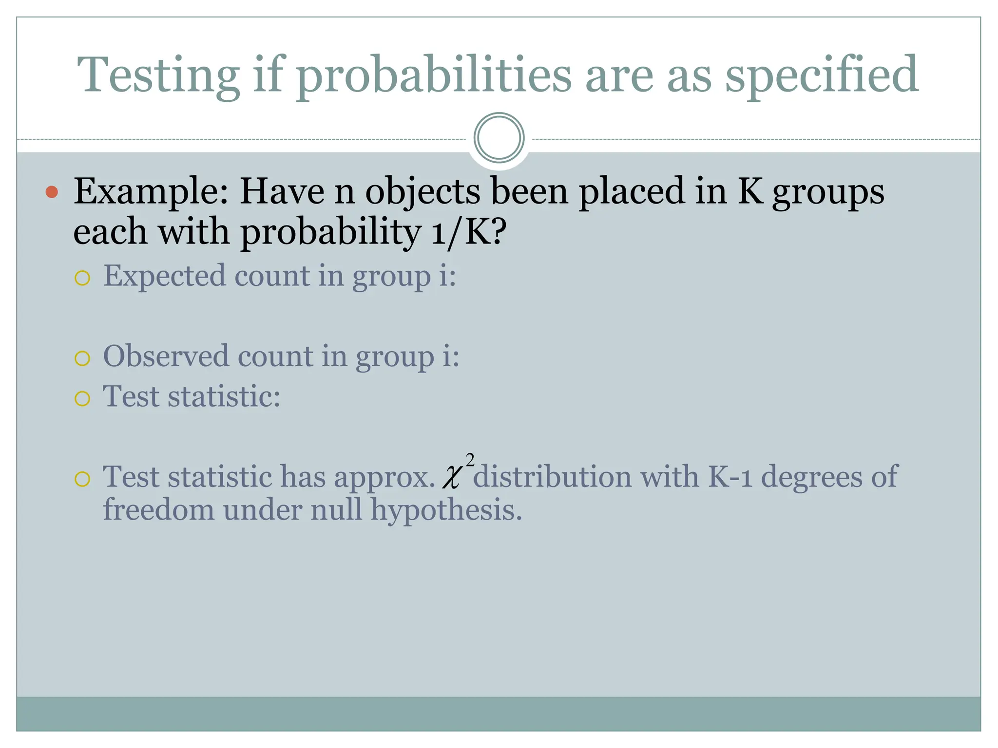
 Example: Have n objects been placed in K groups
each with probability 1/K?
 Expected count in group i:
 Observed count in group i:
 Test statistic:
 Test statistic has approx. distribution with K-1 degrees of
freedom under null hypothesis.
2


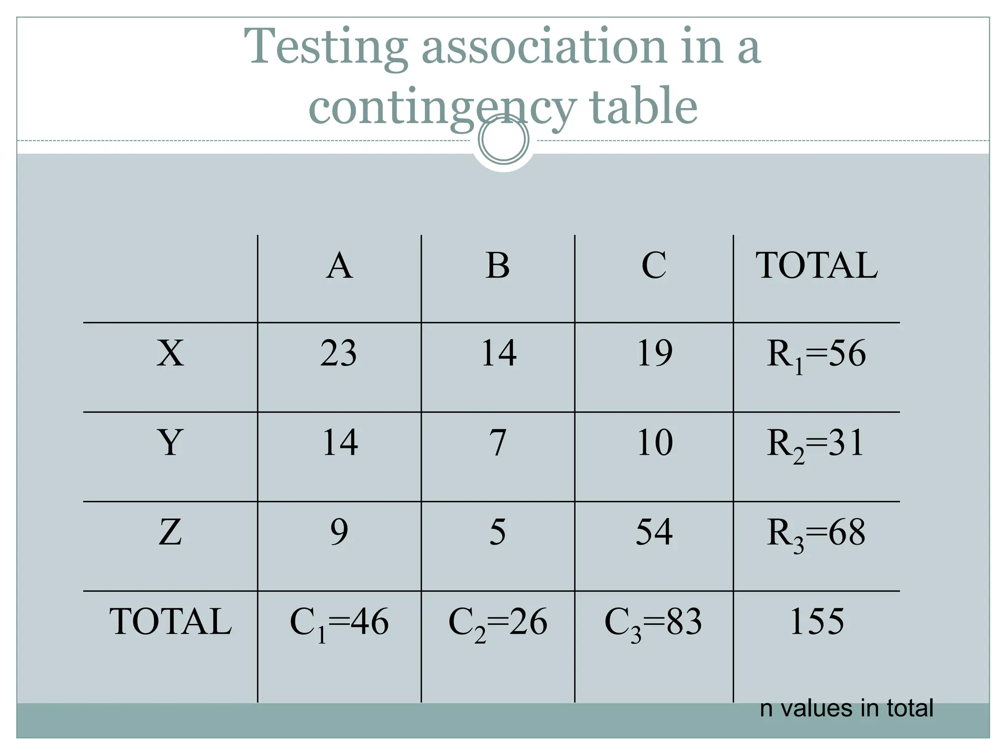
17. Testing association in a
contingency table
A B C TOTAL
X 23 14 19 R1=56
Y 14 7 10 R2=31
Z 9 5 54 R3=68
TOTAL C1=46 C2=26 C3=83 155
n values in total

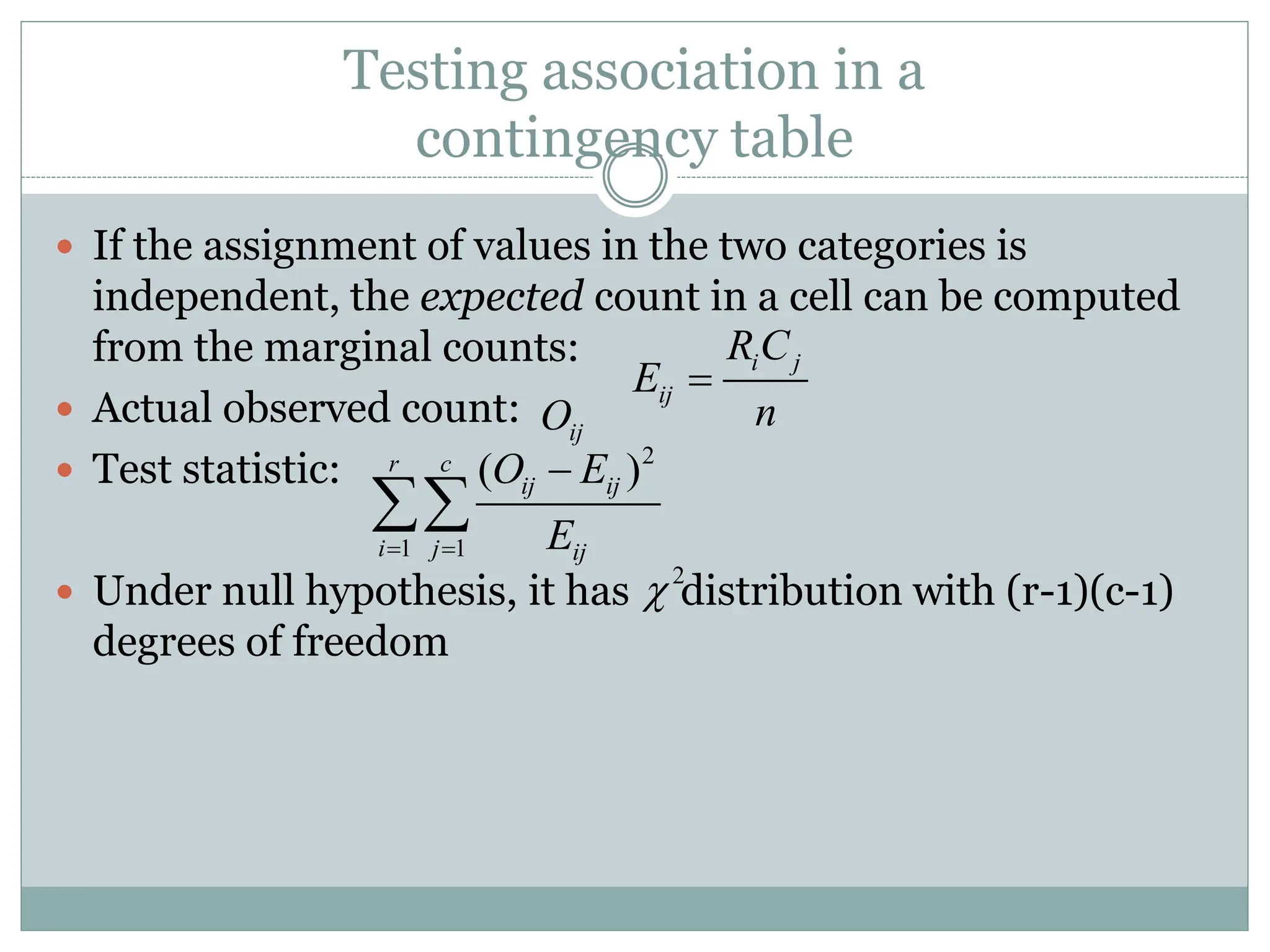
18. Testing association in a
contingency table
 If the assignment of values in the two categories is
independent, the expected count in a cell can be computed
from the marginal counts:
 Actual observed count:
 Test statistic:
 Under null hypothesis, it has distribution with (r-1)(c-1)
degrees of freedom
i j
ij
RC
E
n

ij
O
2
1 1
( )
r c
ij ij
i j ij
O E
E
 


2


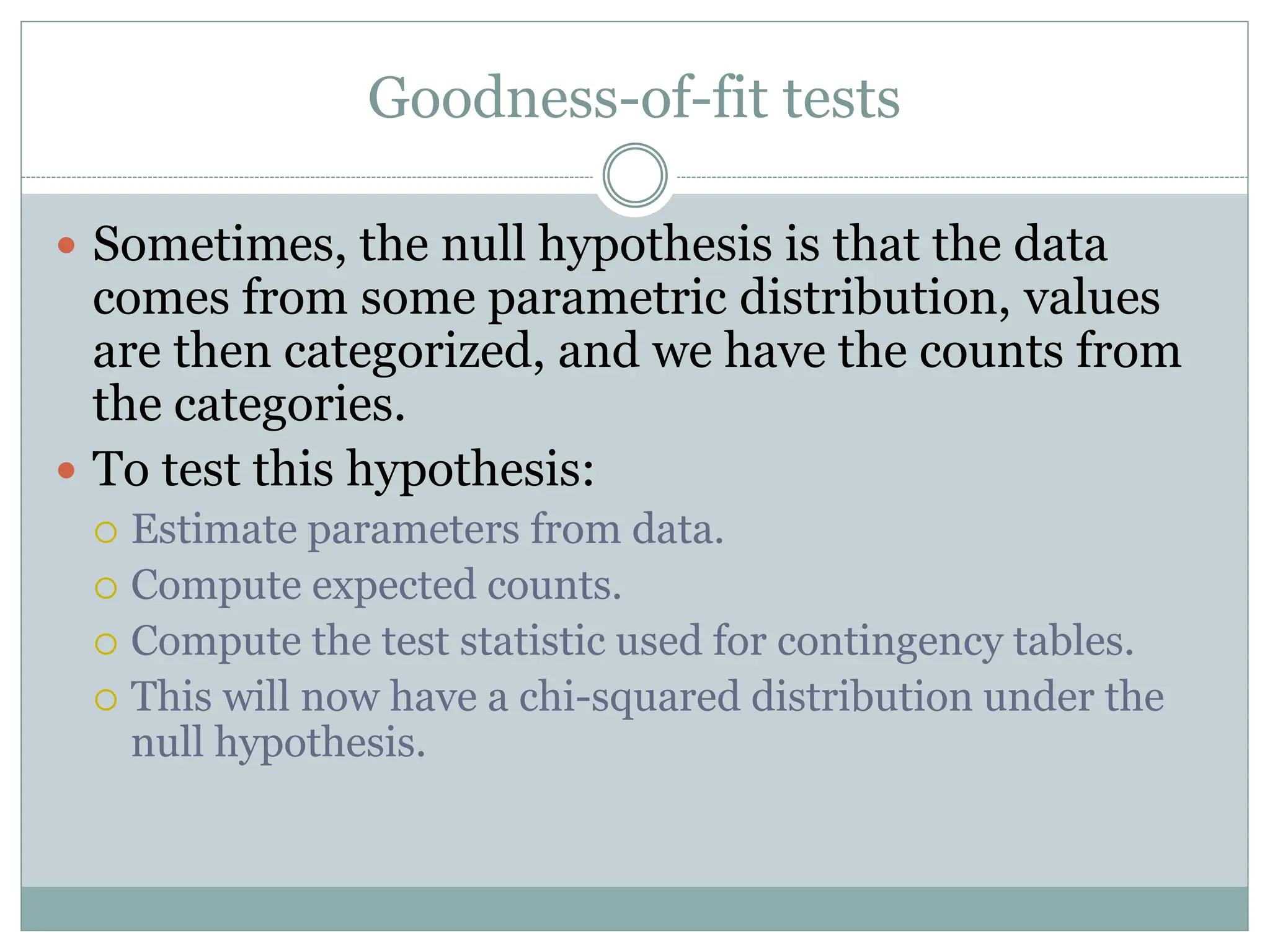
19. Goodness-of-fit tests
 Sometimes, the null hypothesis is that the data
comes from some parametric distribution, values
are then categorized, and we have the counts from
the categories.
 To test this hypothesis:
 Estimate parameters from data.
 Compute expected counts.
 Compute the test statistic used for contingency tables.
 This will now have a chi-squared distribution under the
null hypothesis.

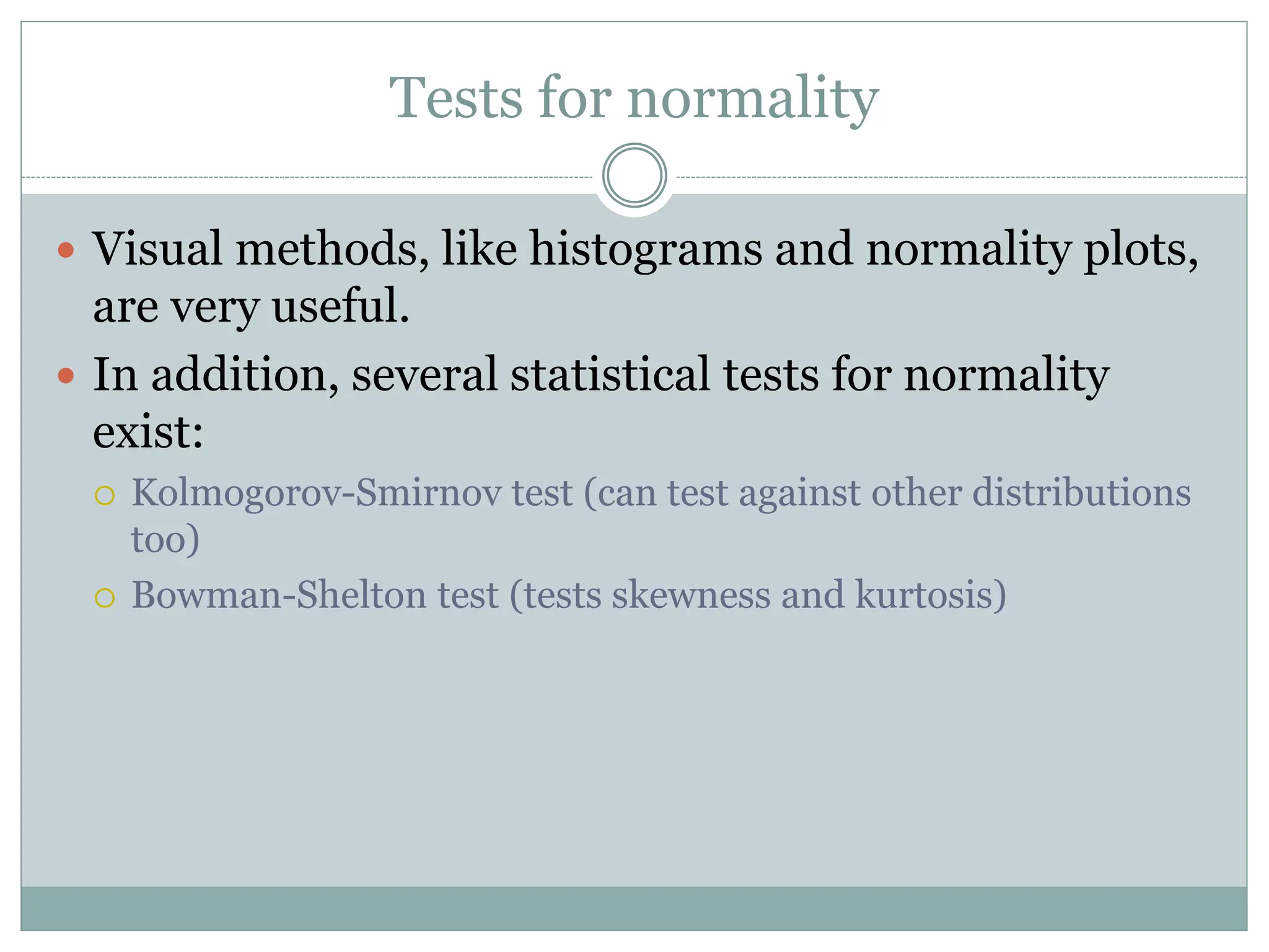
20. Tests for normality
 Visual methods, like histograms and normality plots,
are very useful.
 In addition, several statistical tests for normality
exist:
 Kolmogorov-Smirnov test (can test against other distributions
too)
 Bowman-Shelton test (tests skewness and kurtosis)

21. Remarks on
nonparametric statistics
 Tests with much more general null hypotheses, and
so fewer assumptions
 Often a good choice when normality of the data
cannot be assumed
 If you reject the null hypothesis with a
nonparametric test, it is a robust conclusion
 However, with small amounts of data, you can often
not get significant conclusions

22. Mann-Whitney U test
 This is the nonparametric equivalent of the unpaired
t-test
 It is applied when there are two independent samples
randomly drawn from the population e.g. diabetic patients
versus non-diabetics .
 THe data has to be ordinal i.e. data that can be ranked (put
into order from highest to lowest )
 It is recommended that the data should be >5 and <20 (for
larger samples, use formula or statistical packages)
 The sample size in both population should be equal

23. Uses of Mann-Whitney U test
 Mainly used to analyse the difference between the
medians of two data sets.
 You want to know whether two sets of
measurements genuinely differ.

24. Calculation of Mann-Whitney U test
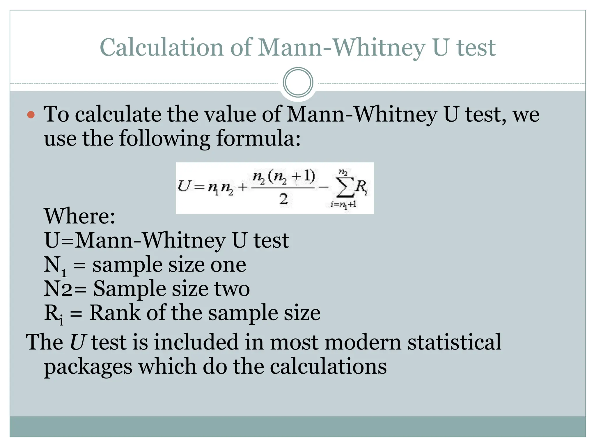
 To calculate the value of Mann-Whitney U test, we
use the following formula:
Where:
U=Mann-Whitney U test
N1 = sample size one
N2= Sample size two
Ri = Rank of the sample size
The U test is included in most modern statistical
packages which do the calculations

25. Mann-Whitney U test
Mann Whitney U-test can be used to compare any two data
sets that are not normally distributed .
As long as the data is capable of being ranked, then the test
can be applied.

26. Analysis of variance
 Comparing more than two groups
 Up to now we have studied situations with
 One observation per object
 One group
 Two groups
 Two or more observations per object
 We will now study situations with one observation
per object, and three or more groups of objects
 The most important question is as usual: Do the
numbers in the groups come from the same
population, or from different populations?

27. ANOVA
 If you have three groups, could plausibly do pairwise
comparisons. But if you have 10 groups? Too many
pairwise comparisons: You would get too many false
positives!
 You would really like to compare a null hypothesis of
all equal, against some difference
 ANOVA: ANalysis Of VAriance

28. One-way ANOVA: Example
 Assume ”treatment results” from 13 patients visiting
one of three doctors are given:
 Doctor A: 24,26,31,27
 Doctor B: 29,31,30,36,33
 Doctor C: 29,27,34,26
 H0: The treatment results are from the same
population of results
 H1: They are from different populations

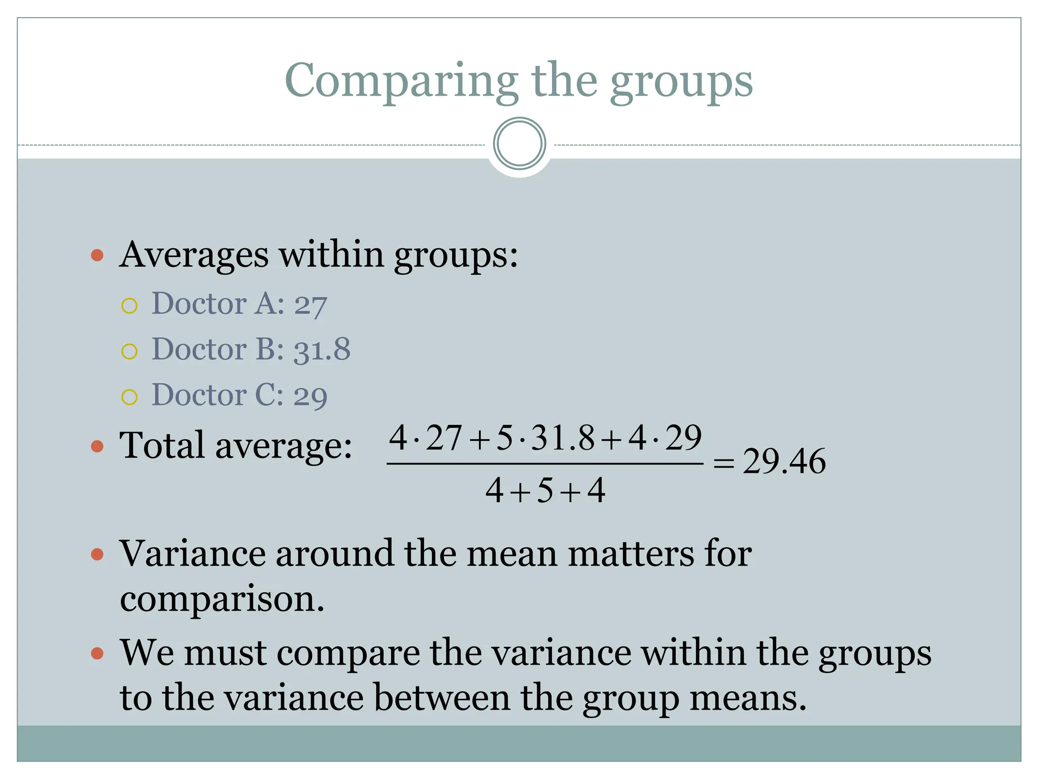
29. Comparing the groups
 Averages within groups:
 Doctor A: 27
 Doctor B: 31.8
 Doctor C: 29
 Total average:
 Variance around the mean matters for
comparison.
 We must compare the variance within the groups
to the variance between the group means.
4 27 5 31.8 4 29
29.46
4 5 4
    

 

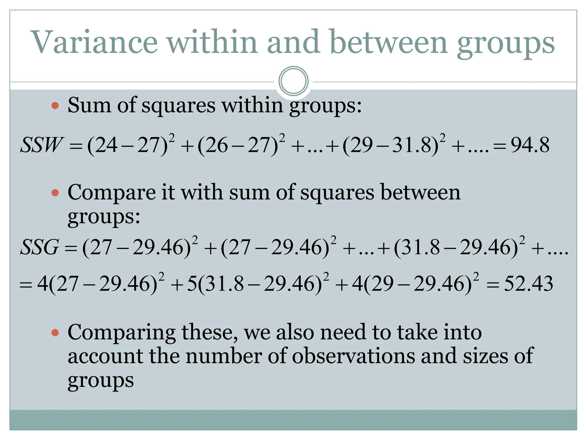
30. Variance within and between groups
 Sum of squares within groups:
 Compare it with sum of squares between
groups:
 Comparing these, we also need to take into
account the number of observations and sizes of
groups
2 2 2
(24 27) (26 27) ... (29 31.8) .... 94.8
SSW         
2 2 2
2 2 2
(27 29.46) (27 29.46) ... (31.8 29.46) ....
4(27 29.46) 5(31.8 29.46) 4(29 29.46) 52.43
SSG        
      

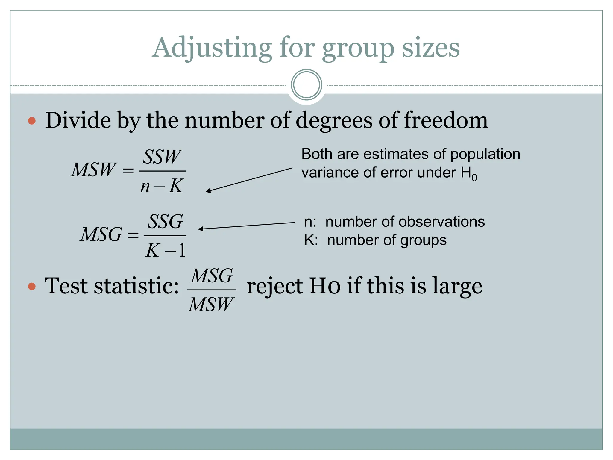
31. Adjusting for group sizes
 Divide by the number of degrees of freedom
 Test statistic: reject H0 if this is large
SSW
MSW
n K


1
SSG
MSG
K


MSG
MSW
Both are estimates of population
variance of error under H0
n: number of observations
K: number of groups

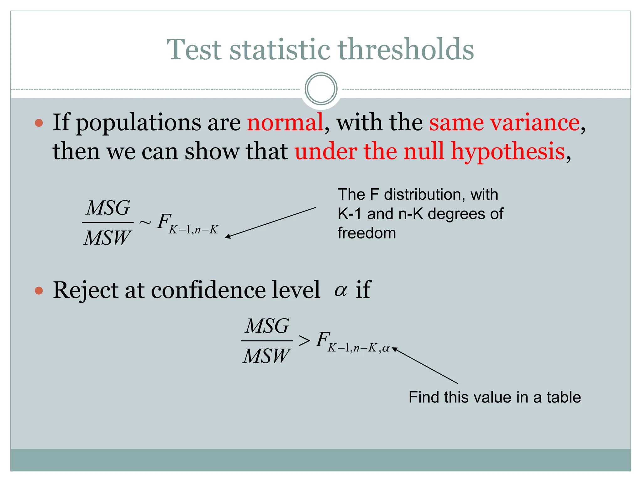
32. Test statistic thresholds
 If populations are normal, with the same variance,
then we can show that under the null hypothesis,
 Reject at confidence level if
1,
~ K n K
MSG
F
MSW
 

1, ,
K n K
MSG
F
MSW

 

The F distribution, with
K-1 and n-K degrees of
freedom
Find this value in a table

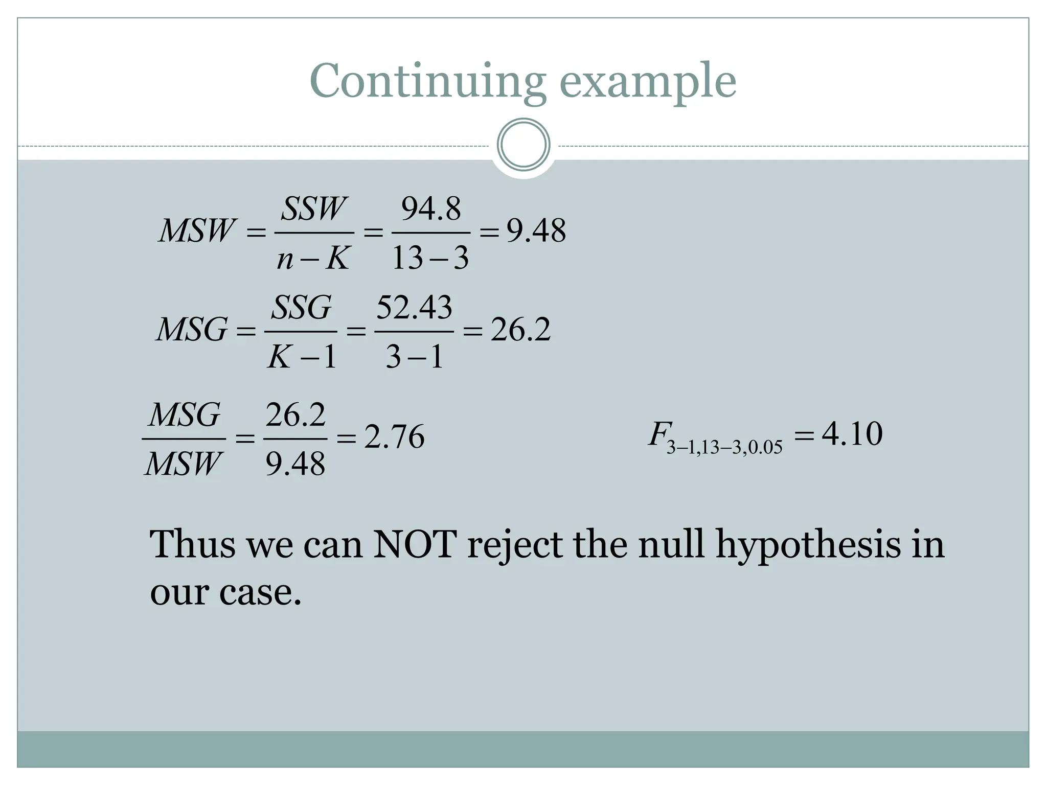
33. Continuing example
Thus we can NOT reject the null hypothesis in
our case.
94.8
9.48
13 3
SSW
MSW
n K
  
 
52.43
26.2
1 3 1
SSG
MSG
K
  
 
26.2
2.76
9.48
MSG
MSW
  3 1,13 3,0.05 4.10
F   

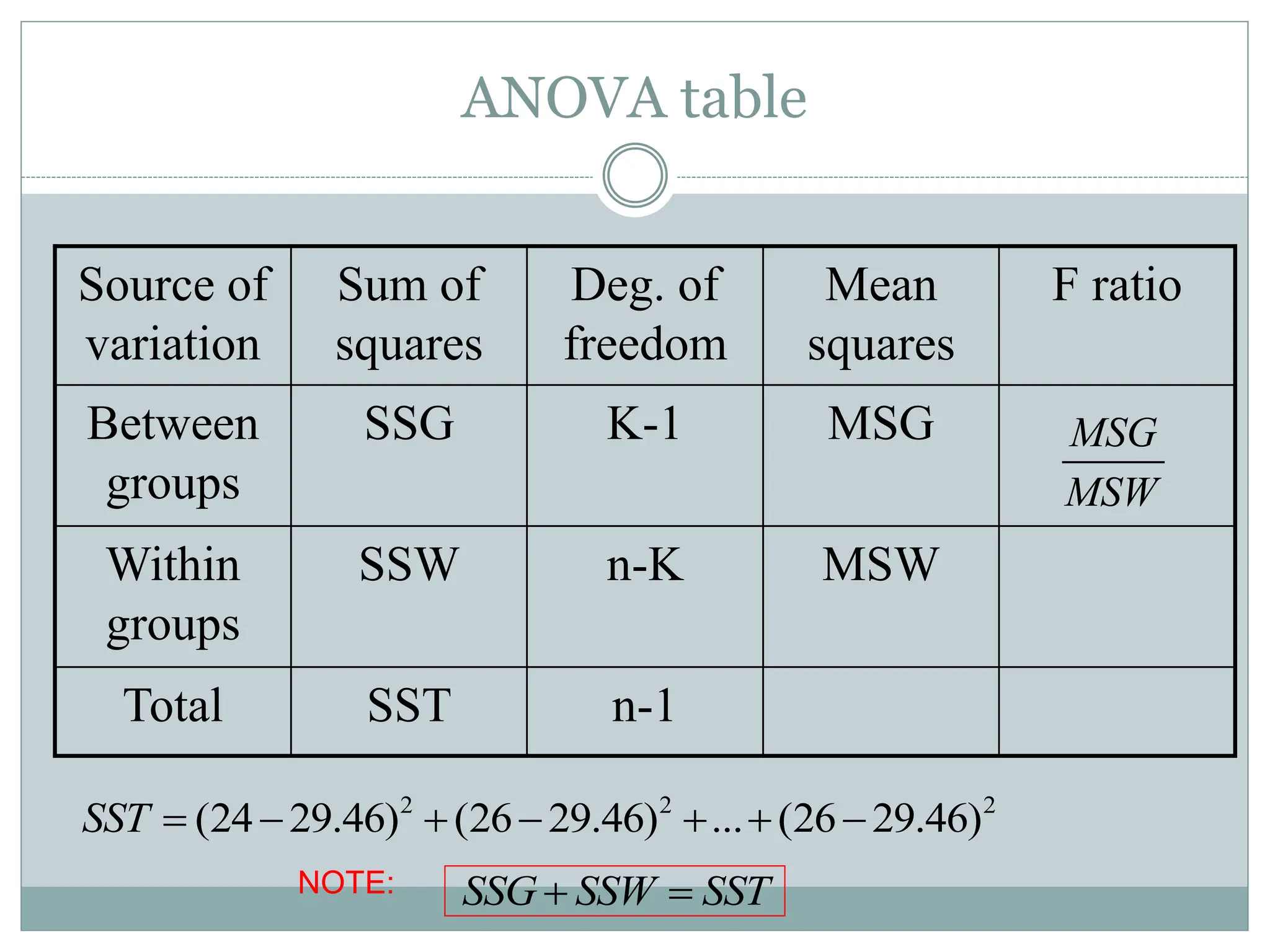
34. ANOVA table
Source of
variation
Sum of
squares
Deg. of
freedom
Mean
squares
F ratio
Between
groups
SSG K-1 MSG
Within
groups
SSW n-K MSW
Total SST n-1
MSG
MSW
2 2 2
(24 29.46) (26 29.46) ... (26 29.46)
SST       
SSG SSW SST
 
NOTE:

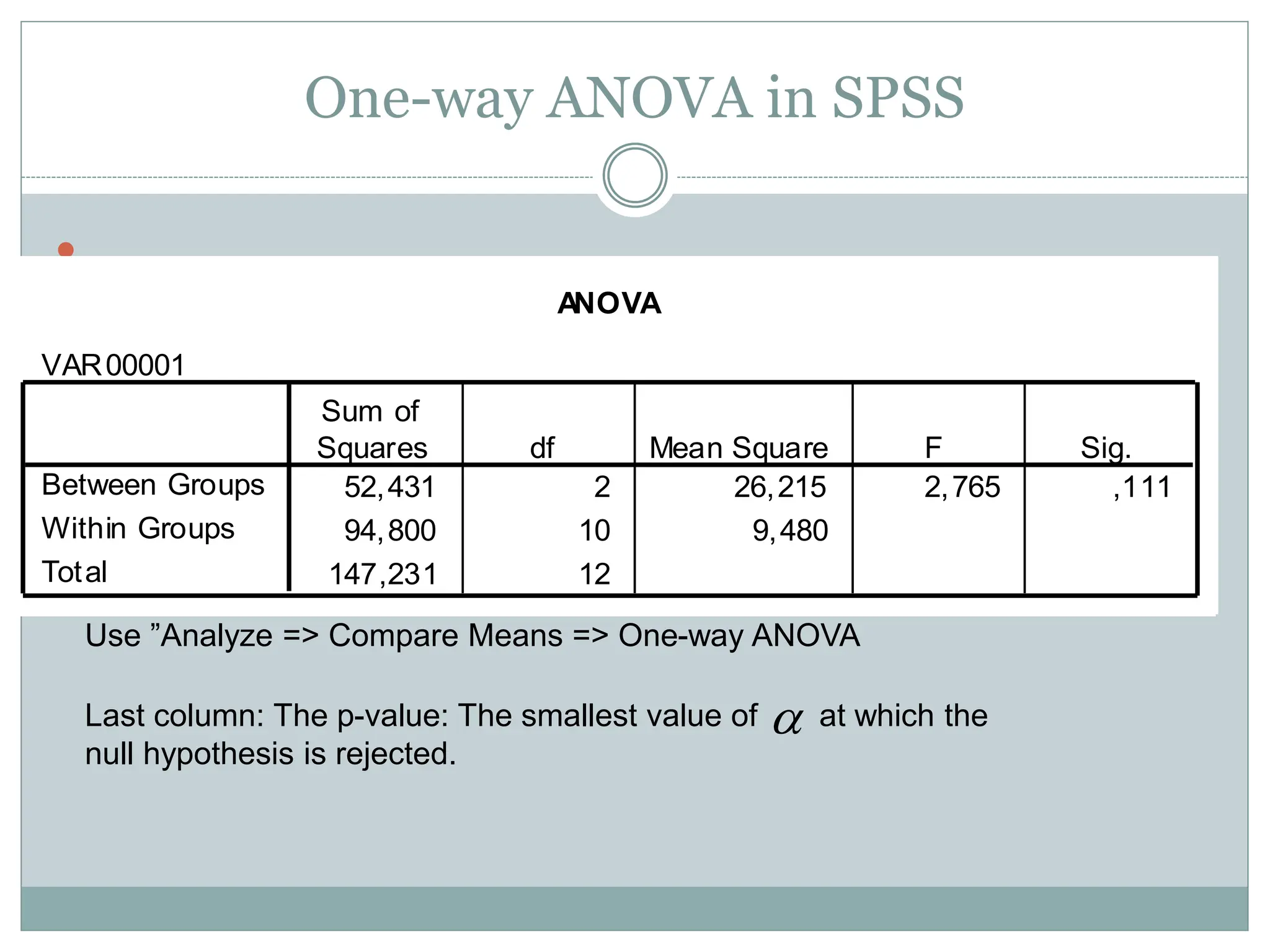
35. One-way ANOVA in SPSS

ANOVA
VAR00001
52,431 2 26,215 2,765 ,111
94,800 10 9,480
147,231 12
Between Groups
Within Groups
Total
Sum of
Squares df Mean Square F Sig.
Use ”Analyze => Compare Means => One-way ANOVA
Last column: The p-value: The smallest value of at which the
null hypothesis is rejected.


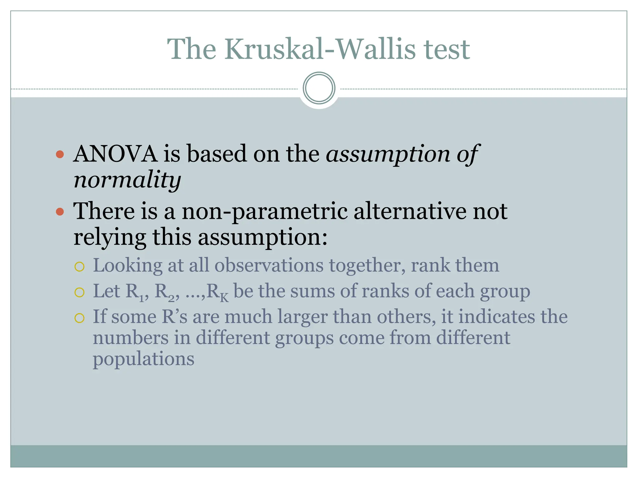
36. The Kruskal-Wallis test
 ANOVA is based on the assumption of
normality
 There is a non-parametric alternative not
relying this assumption:
 Looking at all observations together, rank them
 Let R1, R2, …,RK be the sums of ranks of each group
 If some R’s are much larger than others, it indicates the
numbers in different groups come from different
populations

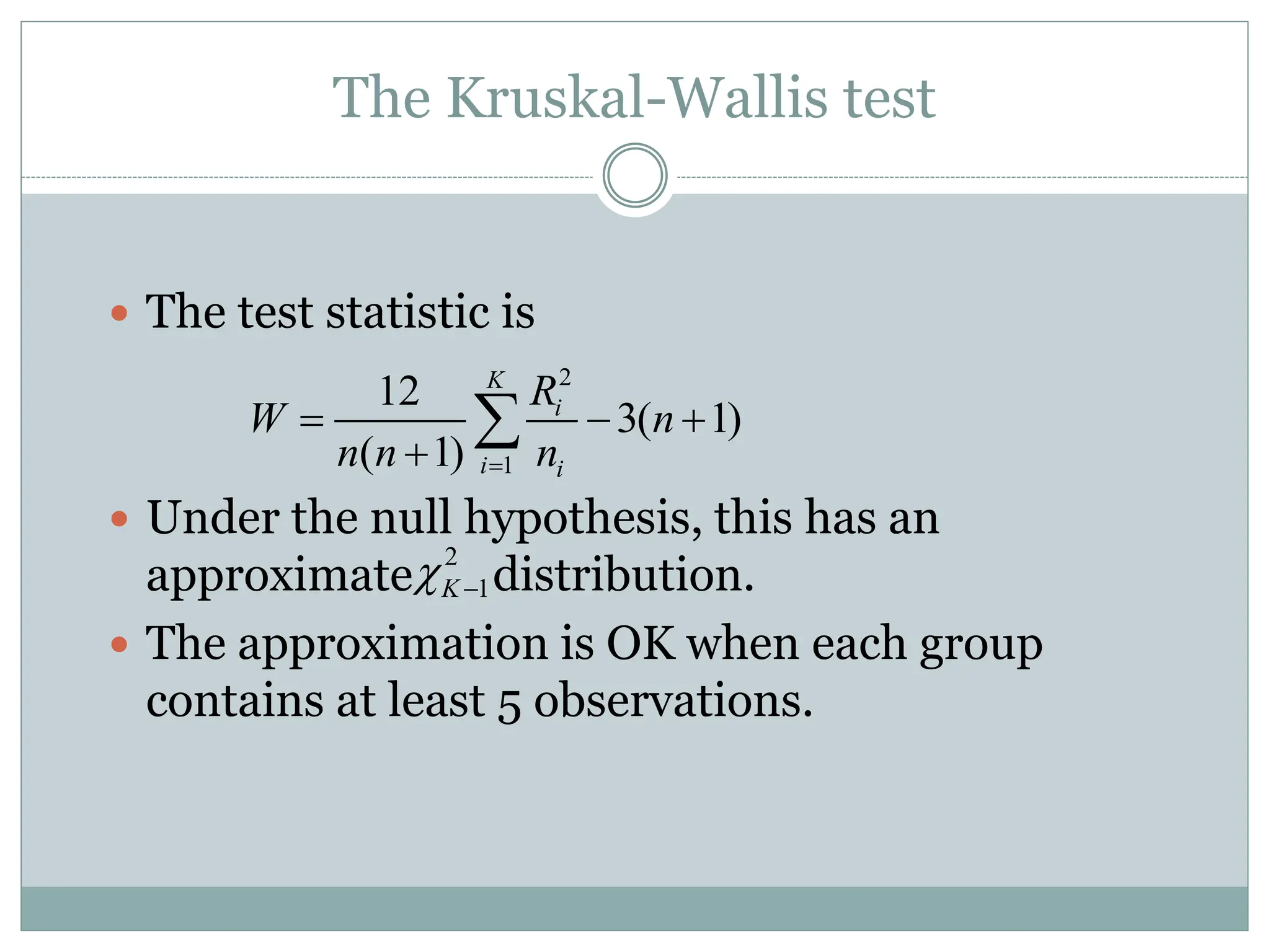
37. The Kruskal-Wallis test
 The test statistic is
 Under the null hypothesis, this has an
approximate distribution.
 The approximation is OK when each group
contains at least 5 observations.
2
1
K
 
2
1
12
3( 1)
( 1)
K
i
i i
R
W n
n n n

  



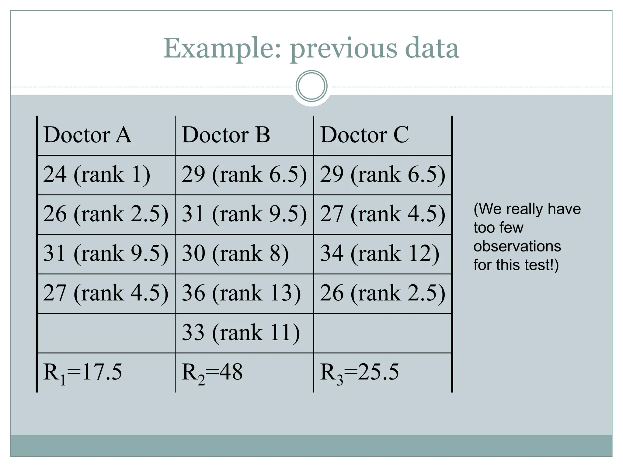
38. Example: previous data
Doctor A Doctor B Doctor C
24 (rank 1) 29 (rank 6.5) 29 (rank 6.5)
26 (rank 2.5) 31 (rank 9.5) 27 (rank 4.5)
31 (rank 9.5) 30 (rank 8) 34 (rank 12)
27 (rank 4.5) 36 (rank 13) 26 (rank 2.5)
33 (rank 11)
R1=17.5 R2=48 R3=25.5
(We really have
too few
observations
for this test!)

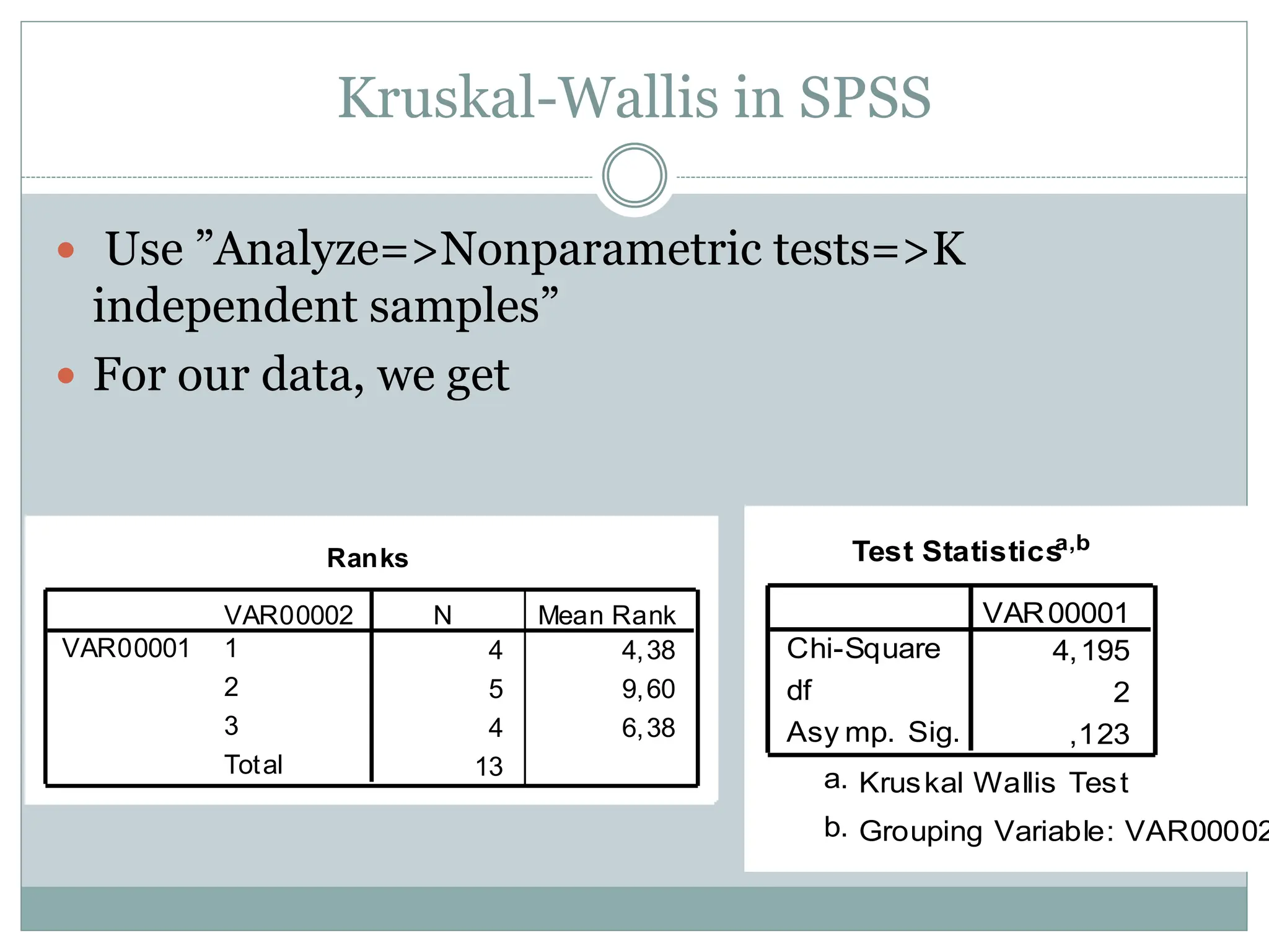
39. Kruskal-Wallis in SPSS
 Use ”Analyze=>Nonparametric tests=>K
independent samples”
 For our data, we get
Ranks
4 4,38
5 9,60
4 6,38
13
VAR00002
1
2
3
Total
VAR00001
N Mean Rank
Test Statistics
a,b
4,195
2
,123
Chi-Square
df
Asy mp. Sig.
VAR00001
Kruskal Wallis Test
a.
Grouping Variable: VAR00002
b.

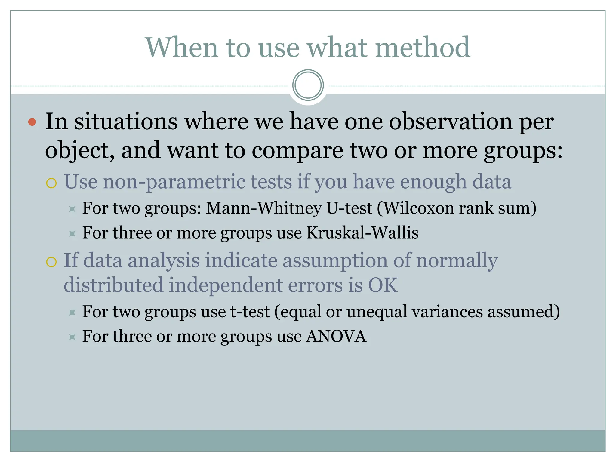
40. When to use what method
 In situations where we have one observation per
object, and want to compare two or more groups:
 Use non-parametric tests if you have enough data
 For two groups: Mann-Whitney U-test (Wilcoxon rank sum)
 For three or more groups use Kruskal-Wallis
 If data analysis indicate assumption of normally
distributed independent errors is OK
 For two groups use t-test (equal or unequal variances assumed)
 For three or more groups use ANOVA

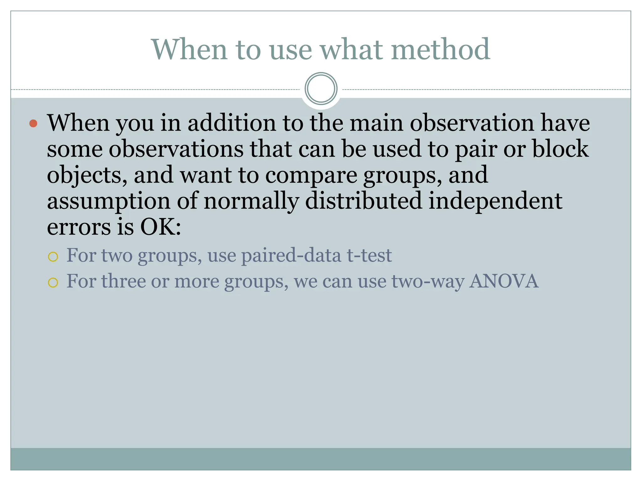
41. When to use what method
 When you in addition to the main observation have
some observations that can be used to pair or block
objects, and want to compare groups, and
assumption of normally distributed independent
errors is OK:
 For two groups, use paired-data t-test
 For three or more groups, we can use two-way ANOVA

42. Two-way ANOVA (without interaction)
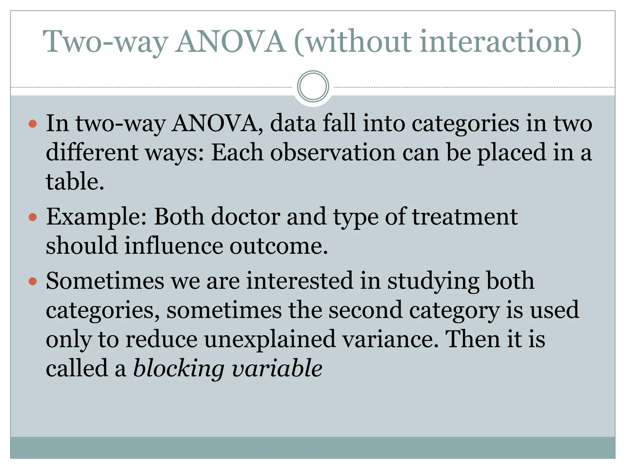
 In two-way ANOVA, data fall into categories in two
different ways: Each observation can be placed in a
table.
 Example: Both doctor and type of treatment
should influence outcome.
 Sometimes we are interested in studying both
categories, sometimes the second category is used
only to reduce unexplained variance. Then it is
called a blocking variable

43. Sums of squares for two-way ANOVA
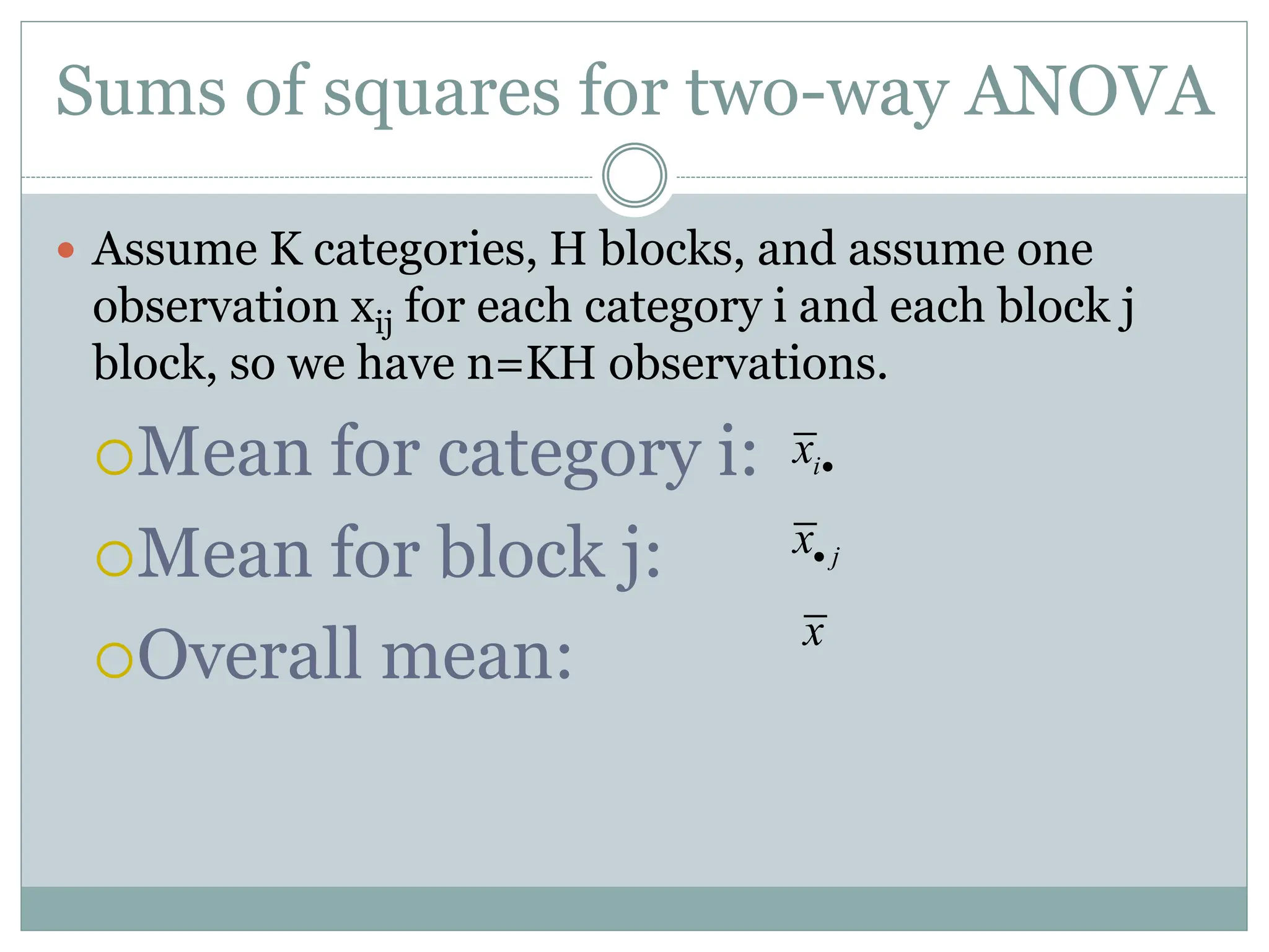
 Assume K categories, H blocks, and assume one
observation xij for each category i and each block j
block, so we have n=KH observations.
Mean for category i:
Mean for block j:
Overall mean:
i
x 
j
x
x

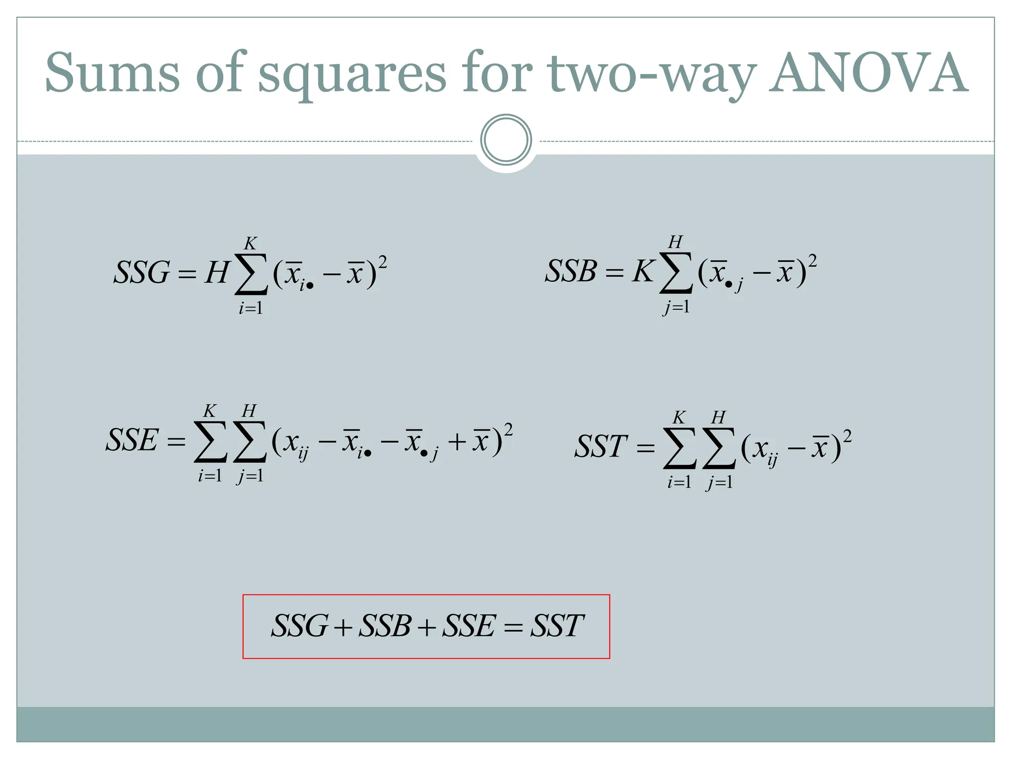
44. Sums of squares for two-way ANOVA
2
1
( )
K
i
i
SSG H x x


 
 2
1
( )
H
j
j
SSB K x x


 

2
1 1
( )
K H
ij i j
i j
SSE x x x x
 
 
   
 2
1 1
( )
K H
ij
i j
SST x x
 
 

SSG SSB SSE SST
  

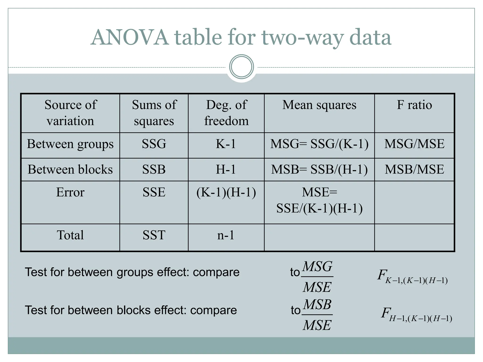
45. ANOVA table for two-way data
Source of
variation
Sums of
squares
Deg. of
freedom
Mean squares F ratio
Between groups SSG K-1 MSG= SSG/(K-1) MSG/MSE
Between blocks SSB H-1 MSB= SSB/(H-1) MSB/MSE
Error SSE (K-1)(H-1) MSE=
SSE/(K-1)(H-1)
Total SST n-1
Test for between groups effect: compare to
Test for between blocks effect: compare to
MSG
MSE
MSB
MSE
1,( 1)( 1)
K K H
F   
1,( 1)( 1)
H K H
F   

46. Two-way ANOVA (with interaction)
 The setup above assumes that the blocking variable
influences outcomes in the same way in all categories
(and vice versa)
 We can check if there is interaction between the
blocking variable and the categories by extending the
model with an interaction term

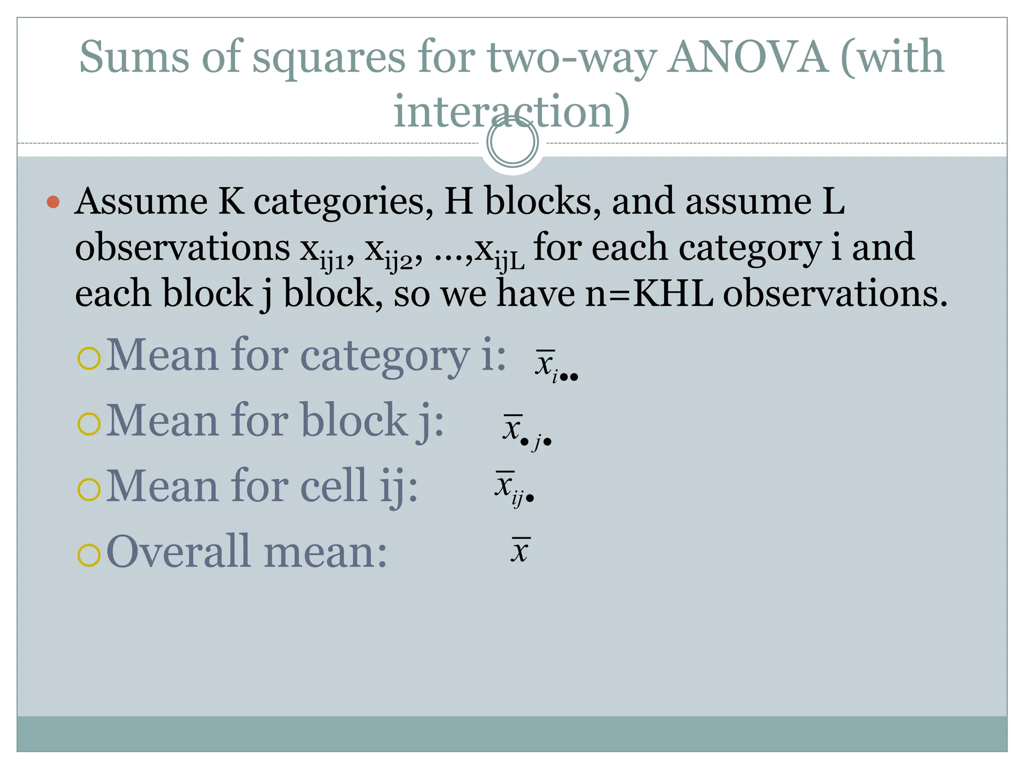
47. Sums of squares for two-way ANOVA (with
interaction)
 Assume K categories, H blocks, and assume L
observations xij1, xij2, …,xijL for each category i and
each block j block, so we have n=KHL observations.
Mean for category i:
Mean for block j:
Mean for cell ij:
Overall mean:
i
x 
j
x 
x
ij
x 

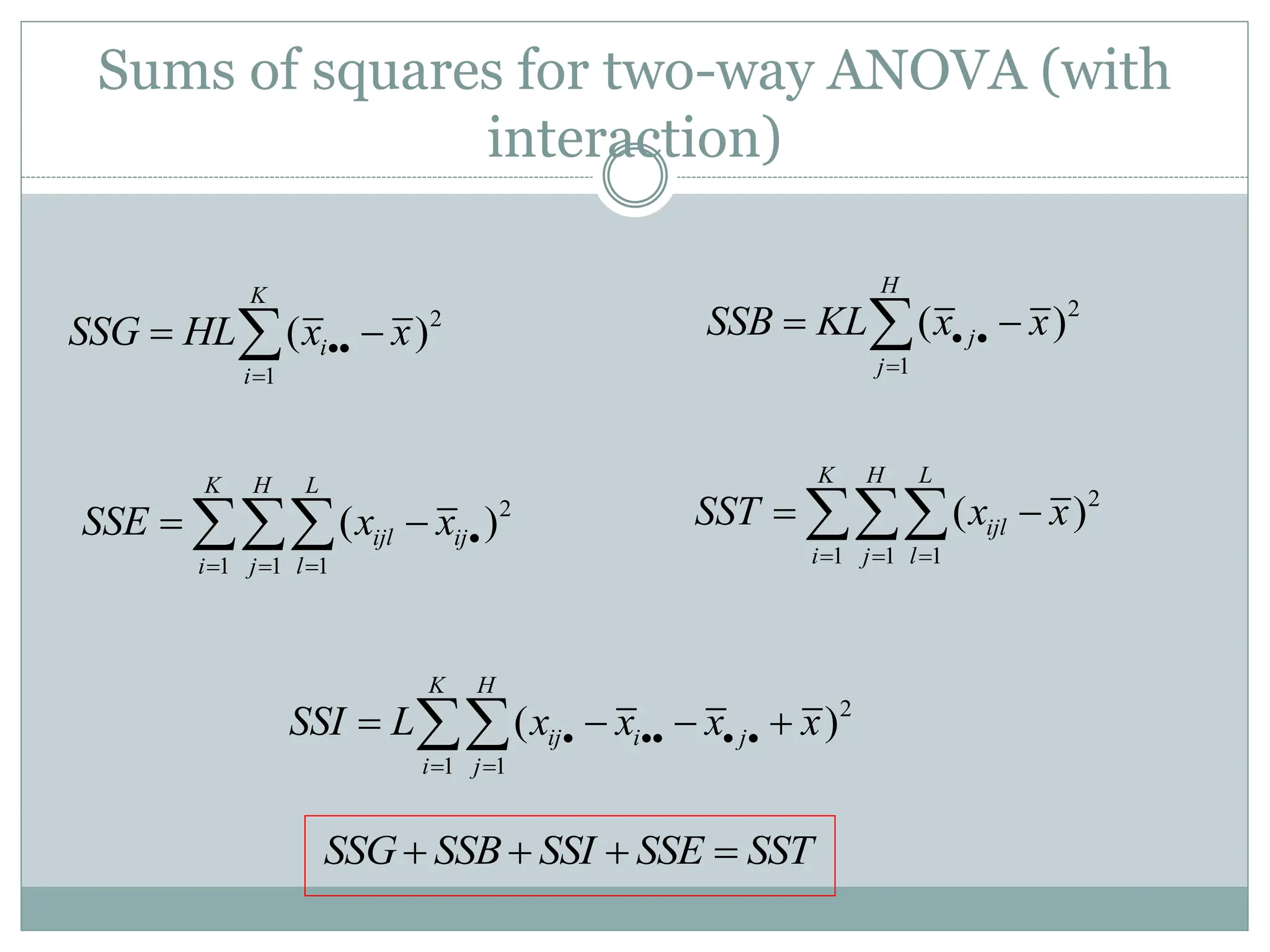
48. Sums of squares for two-way ANOVA (with
interaction)
2
1
( )
K
i
i
SSG HL x x


 

2
1
( )
H
j
j
SSB KL x x
 

 

2
1 1
( )
K H
ij i j
i j
SSI L x x x x
   
 
   

2
1 1 1
( )
K H L
ijl
i j l
SST x x
  
 

SSG SSB SSI SSE SST
   
2
1 1 1
( )
K H L
ijl ij
i j l
SSE x x 
  
 


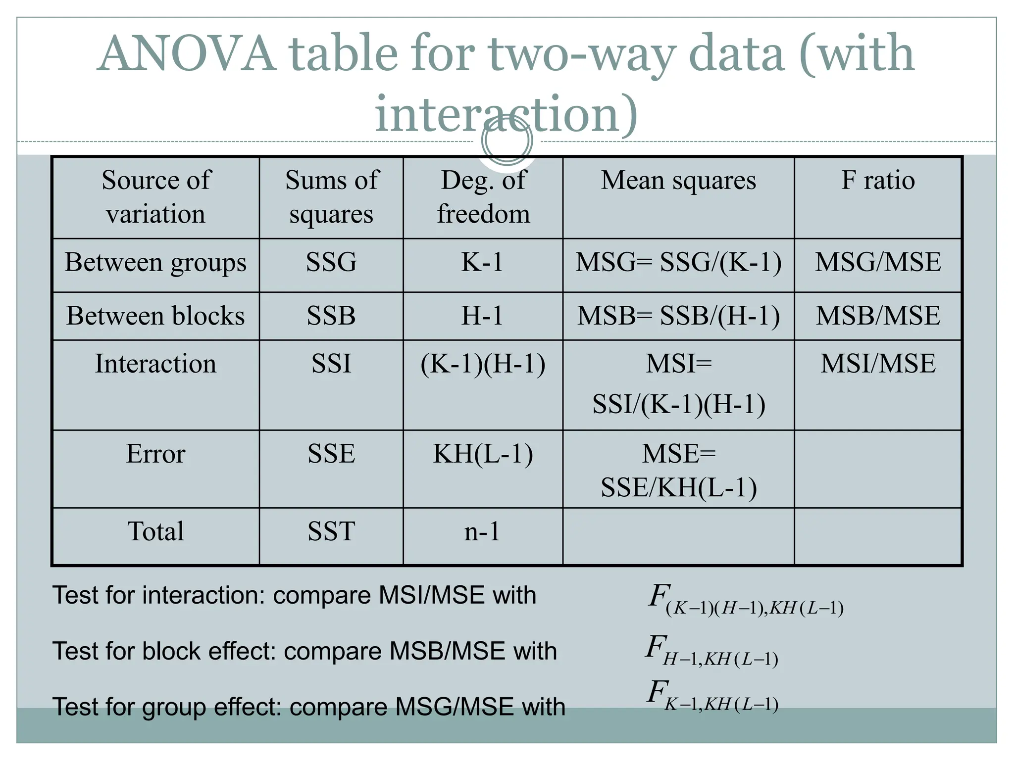
49. ANOVA table for two-way data (with
interaction)
Source of
variation
Sums of
squares
Deg. of
freedom
Mean squares F ratio
Between groups SSG K-1 MSG= SSG/(K-1) MSG/MSE
Between blocks SSB H-1 MSB= SSB/(H-1) MSB/MSE
Interaction SSI (K-1)(H-1) MSI=
SSI/(K-1)(H-1)
MSI/MSE
Error SSE KH(L-1) MSE=
SSE/KH(L-1)
Total SST n-1
Test for interaction: compare MSI/MSE with
Test for block effect: compare MSB/MSE with
Test for group effect: compare MSG/MSE with 1, ( 1)
K KH L
F  
1, ( 1)
H KH L
F  
( 1)( 1), ( 1)
K H KH L
F   

50. Notes on ANOVA
 All analysis of variance (ANOVA) methods are based
on the assumptions of normally distributed and
independent errors
 The same problems can be described using the
regression framework. We get exactly the same tests
and results!
 There are many extensions beyond those mentioned

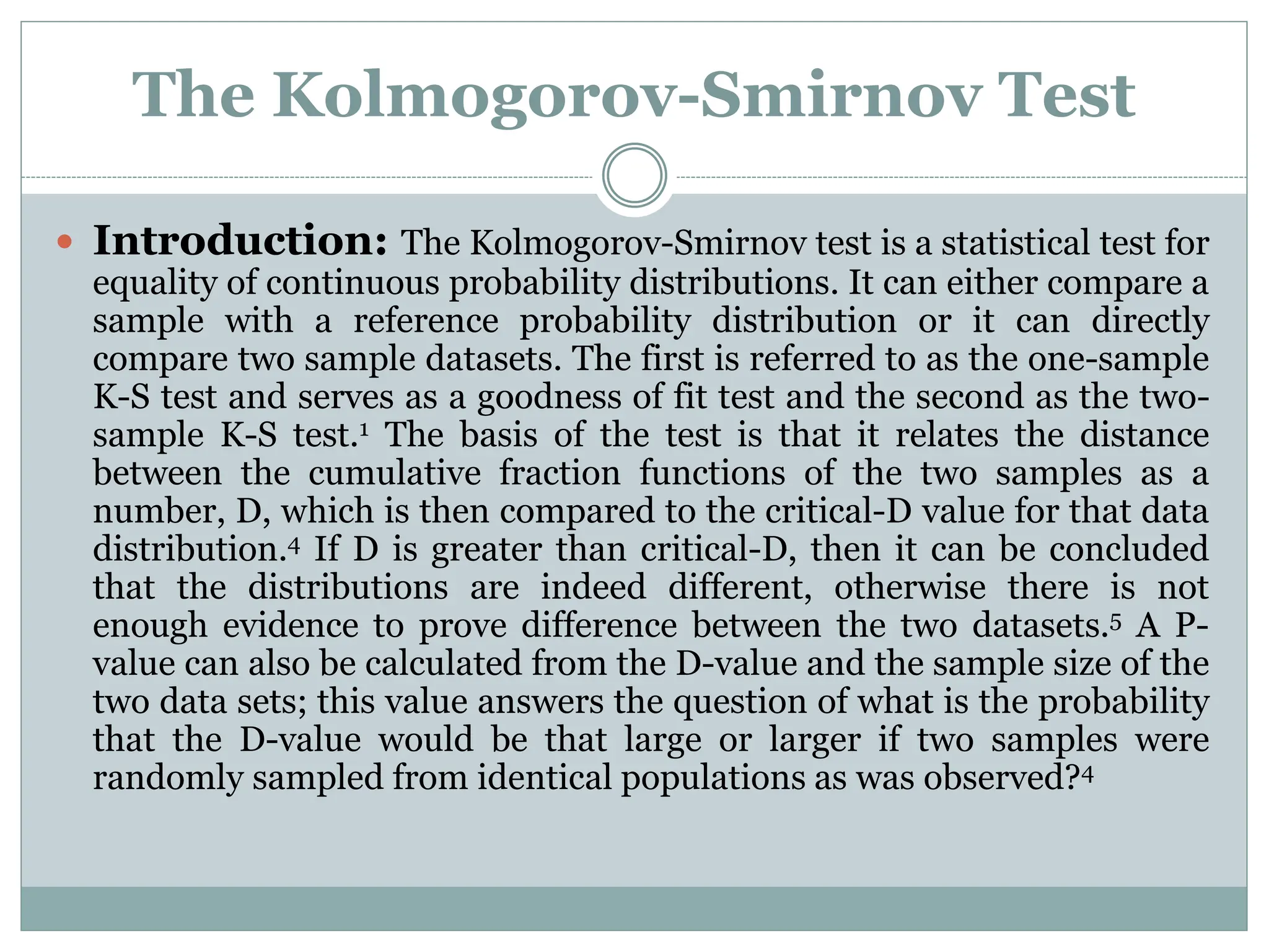
51. The Kolmogorov-Smirnov Test
 Introduction: The Kolmogorov-Smirnov test is a statistical test for
equality of continuous probability distributions. It can either compare a
sample with a reference probability distribution or it can directly
compare two sample datasets. The first is referred to as the one-sample
K-S test and serves as a goodness of fit test and the second as the two-
sample K-S test.1 The basis of the test is that it relates the distance
between the cumulative fraction functions of the two samples as a
number, D, which is then compared to the critical-D value for that data
distribution.4 If D is greater than critical-D, then it can be concluded
that the distributions are indeed different, otherwise there is not
enough evidence to prove difference between the two datasets.5 A P-
value can also be calculated from the D-value and the sample size of the
two data sets; this value answers the question of what is the probability
that the D-value would be that large or larger if two samples were
randomly sampled from identical populations as was observed?4

52. VALUES OF DATA SET 1 AND DATA SET 2

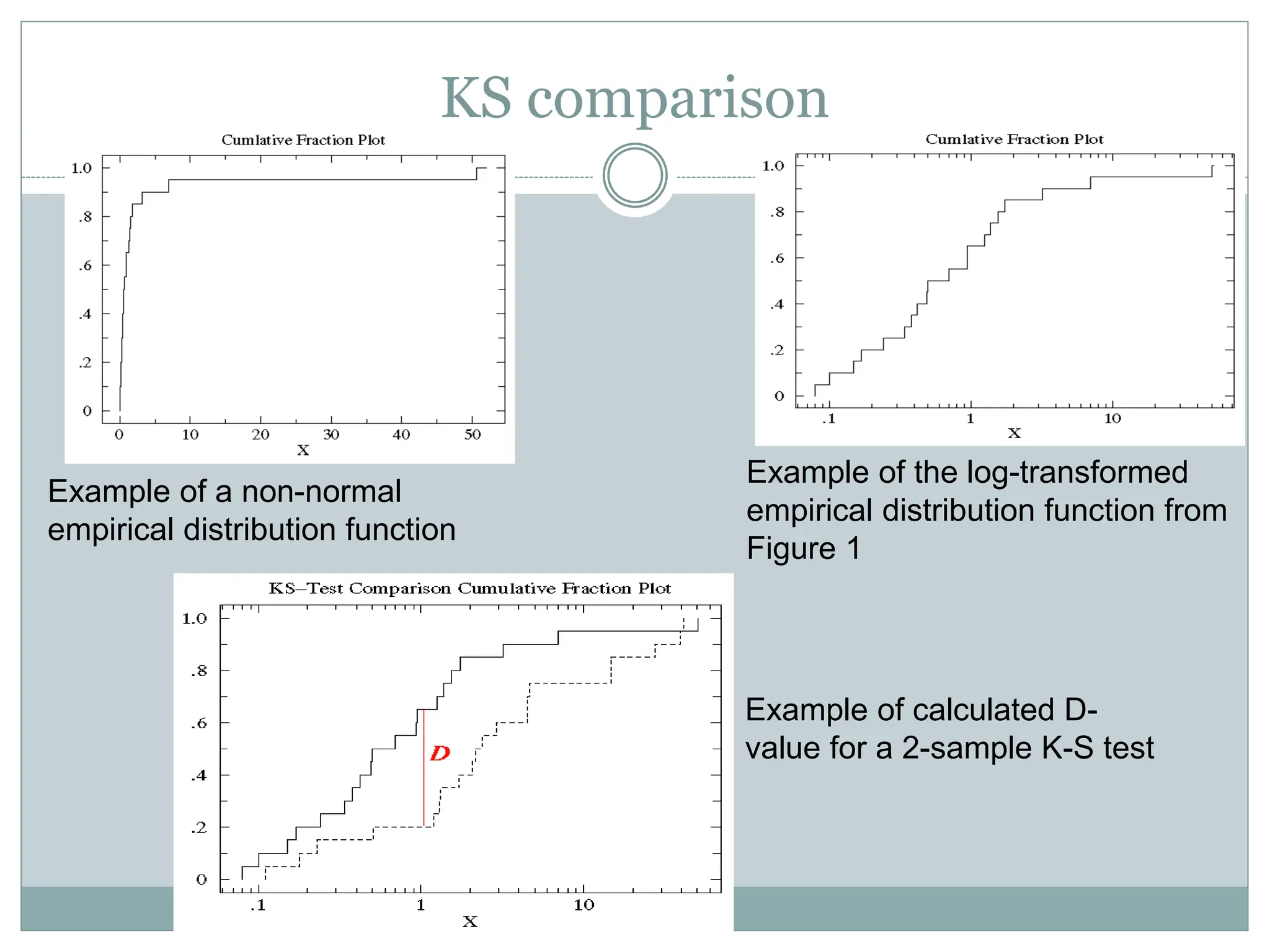
53. KS comparison
Example of a non-normal
empirical distribution function
Example of the log-transformed
empirical distribution function from
Figure 1
Example of calculated D-
value for a 2-sample K-S test

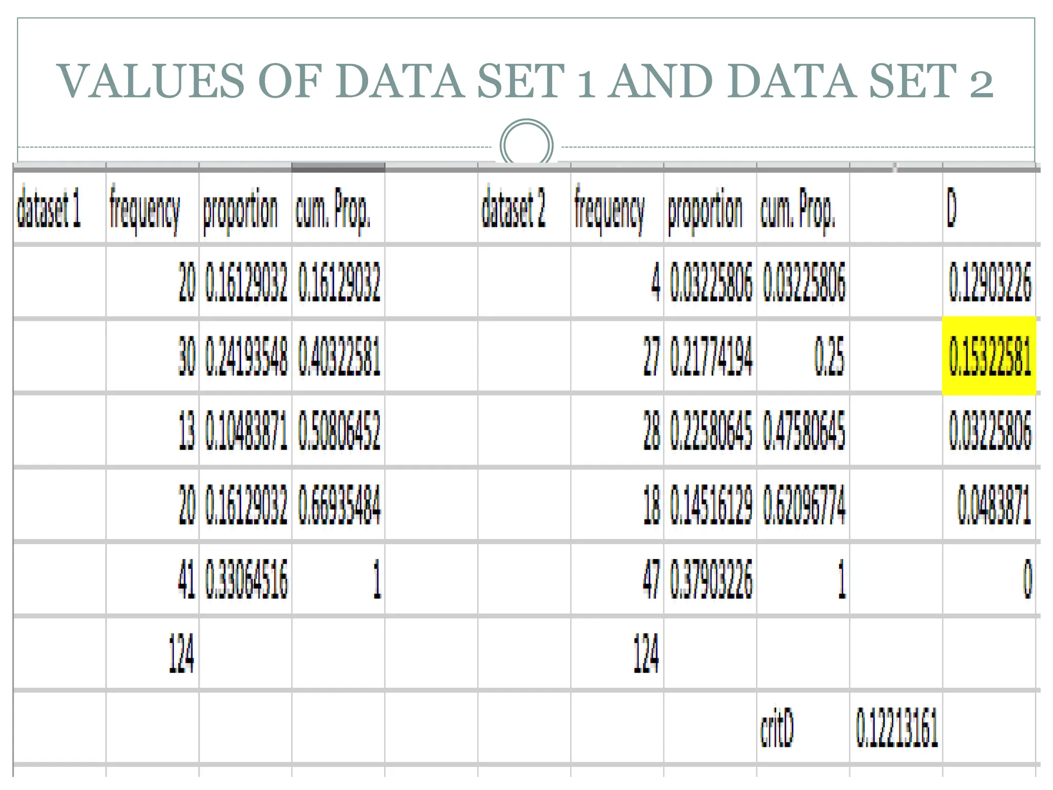
54. Procedure:
 1. Order data sets from smallest to largest.
 2. For each value in the data sets, calculate the percent of data
strictly smaller than that value.
 3.Plot all calculated percent values as steps on a cumulative fraction
function, one for each data set if it is a two-sample K-S test.
 4.If steps are bunched close to one another on one side of the graph,
you can take the log of all data points and plot the distribution
function based on that instead. For log, all data points must be
nonzero and nonnegative.
 5. Calculate the maximum vertical distance between the two
functions to acquire the D-value. This value along with the
corresponding P-value states whether data sets differ significantly.

55. Strengths of the K-S test:
 1. It is nonparametric.
 2. D-value result will not change if X values are
transformed to logs or reciprocals or any other
transformation.
 3. No restriction on sample size.
 4. The D-value is easy to compute and the graph
can be understood easily.
 5. One sample K-S test can serve as a goodness-of-
fit test and can link data and theory.

56. Drawbacks:
1. The K-S test is less sensitive when the
differences between curves is greatest at the
beginning or the end of the distributions. It
works best when EDFs deviate the most near
the center of the distribution.
2. The K-S test cannot be applied in two or more
dimensions because it is a EDF based test.