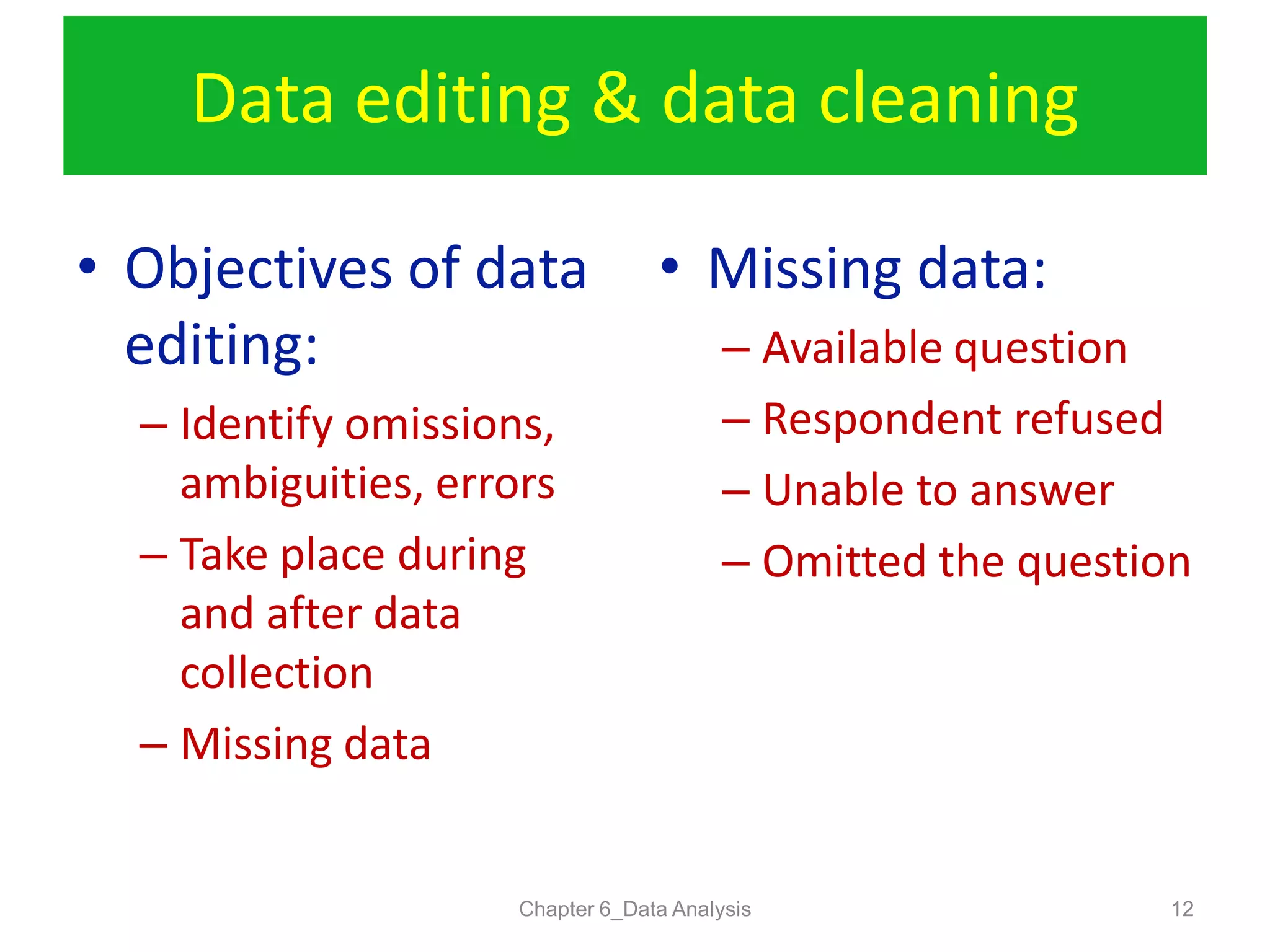
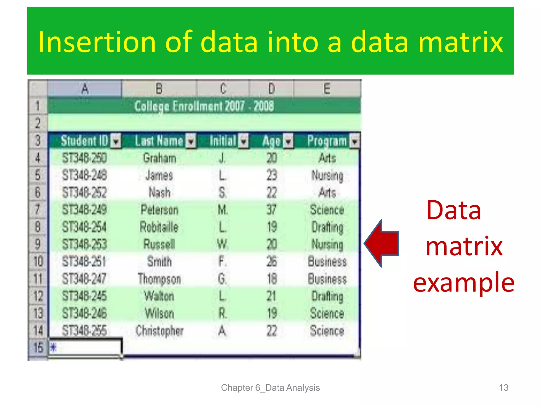
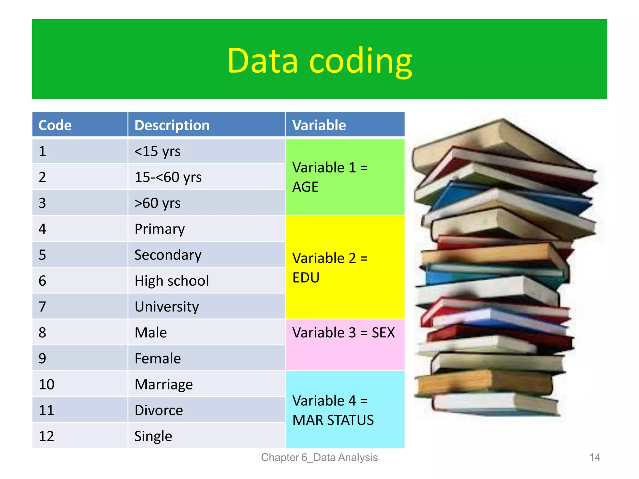
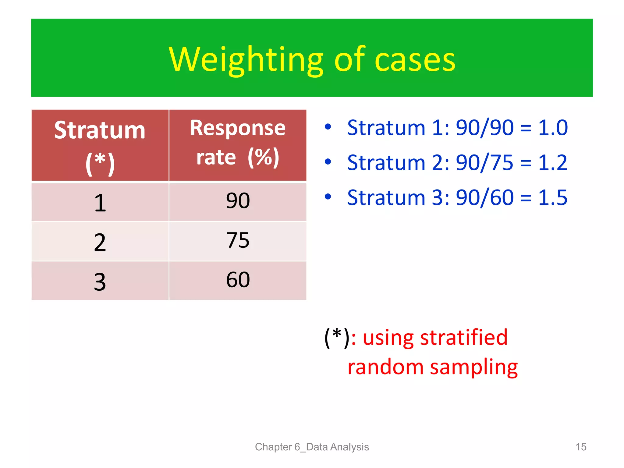
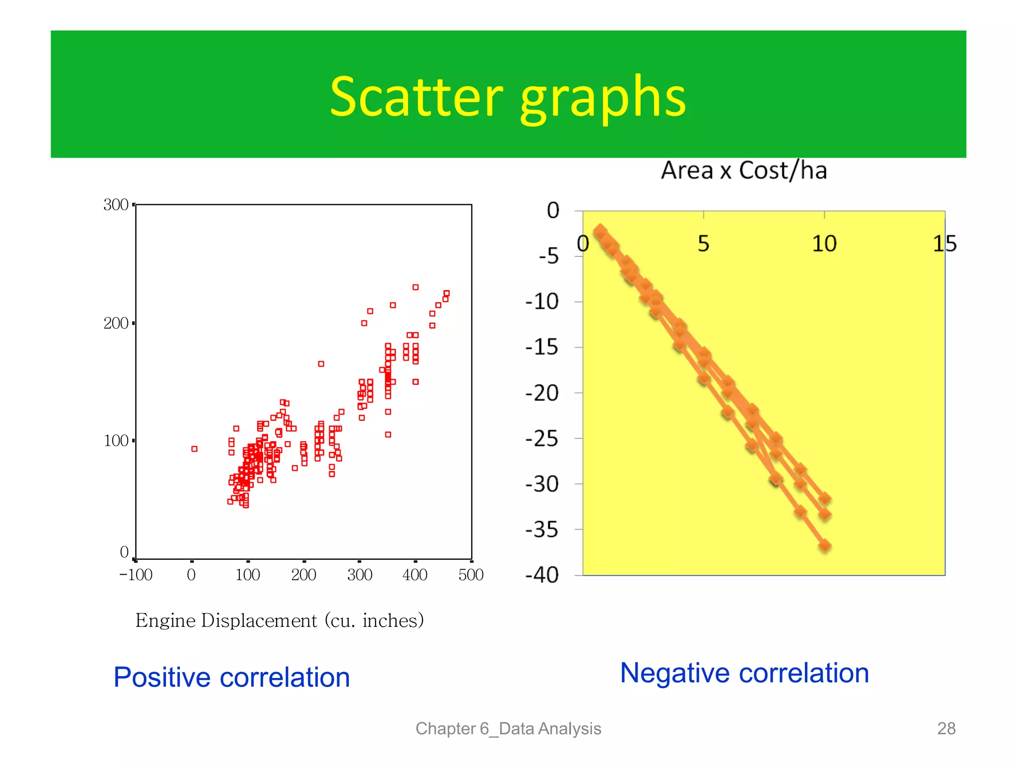
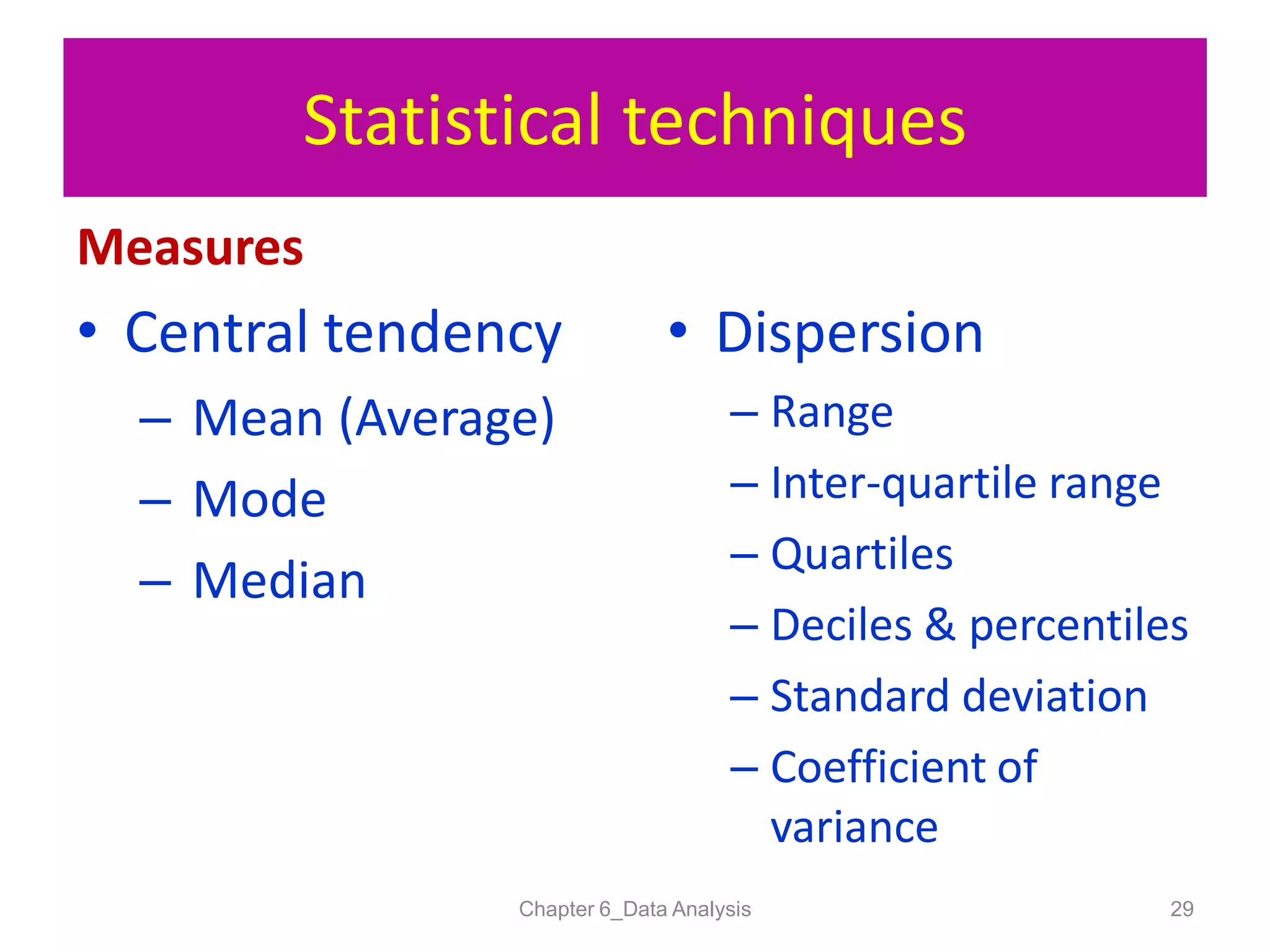
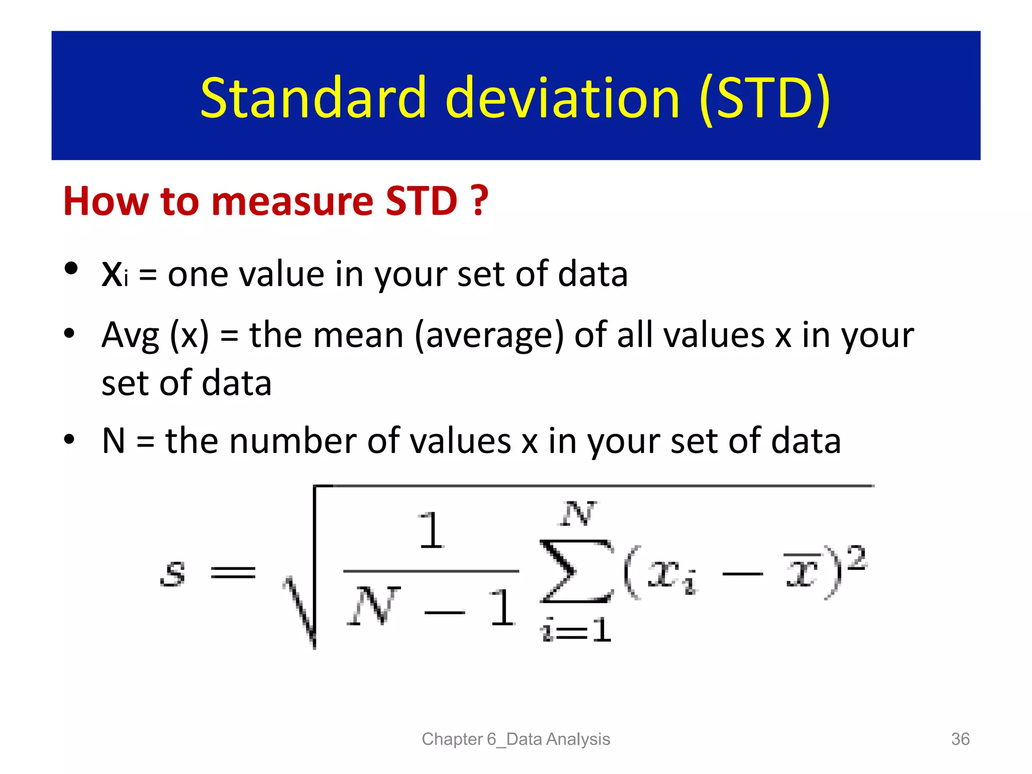
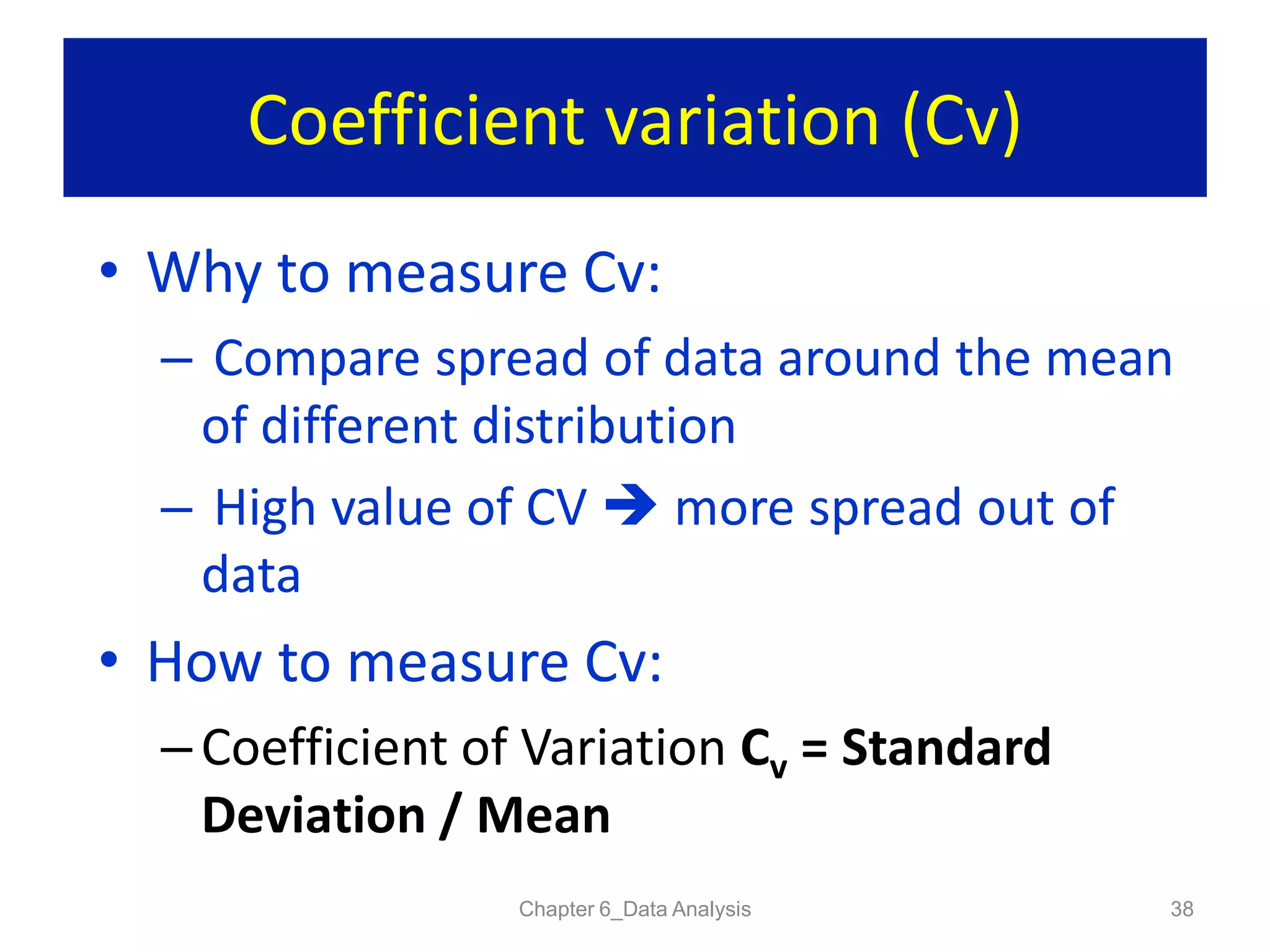
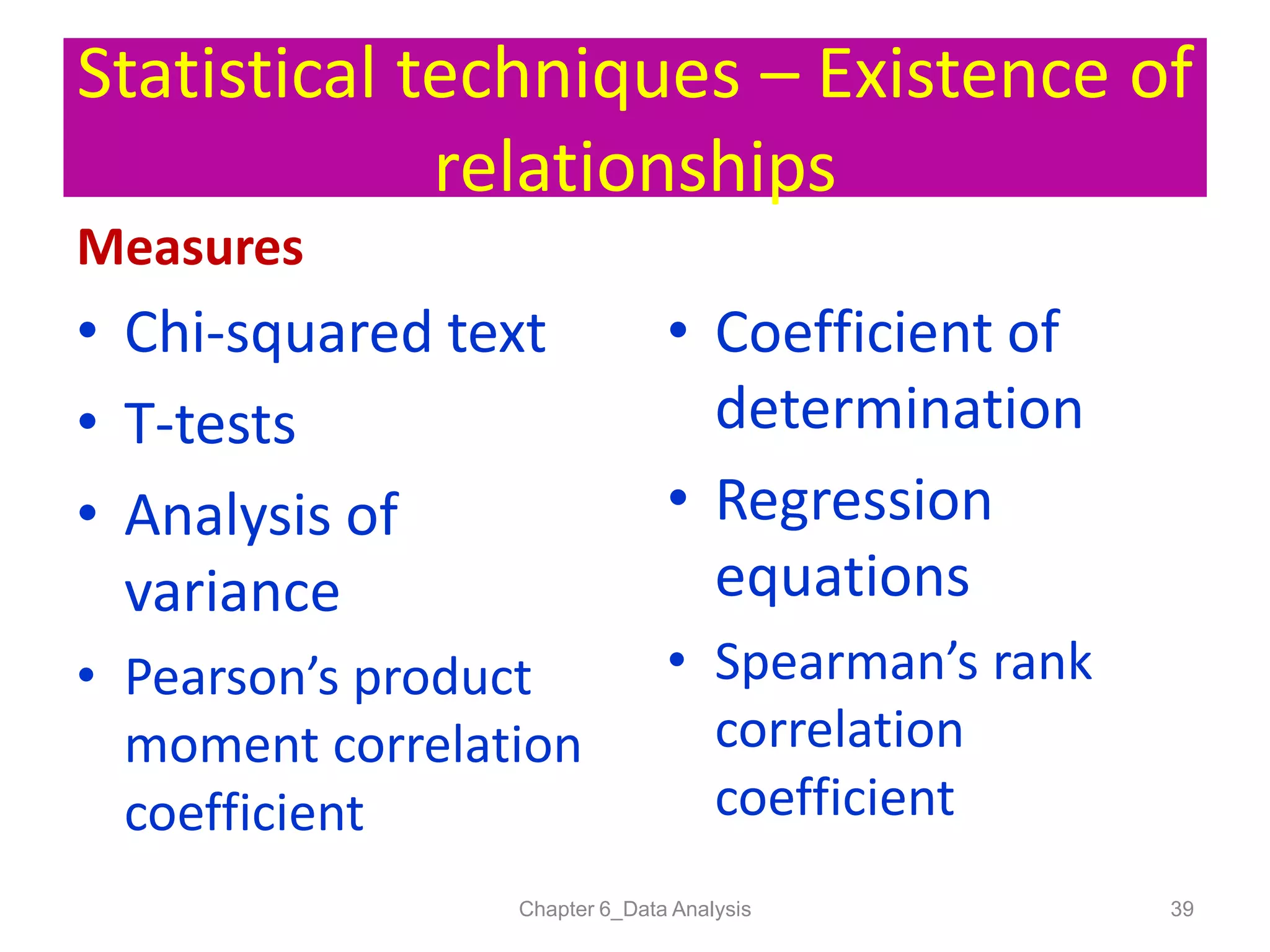
RESEARCH PROJECT
Data
Analysis
1Chapter 6_Data Analysis
Lecturer: Ho Cao Viet (PhD)
6
Student should be able to understand:
How to prepare data for analysis
1
3
2
4
2Chapter 6_Data Analysis
Learning objectives
Type of qualitative data
The use of graph in data analysis
The use of statistical techniques in
data analysis
5 How to analyze qualitative data
Classification of Quantitative Data
Categorical
3Chapter 6_Data Analysis
Quantifiable
Nominal Ordinal Discrete Continuous
Interval Ratio
Quantitative Data
Nominal & Ordinal Data
• Nominal data (Descriptive data):
– Cannot be measured numerically
– Can be categorized
• Ordinal data (Ranked data):
– Ex: results of class mathematics test  no
individual scores  place students in rank
order
Chapter 6_Data Analysis 4
Quantifiable Data
• Can be measured numerically as qualities
• Have individual numerical values
• Discrete data: be measured accurately on a
scale/whole numbers
– Ex: number of illness person, number of goals
• Continuous data: take on any value
– Ex: temperature in HCMC, scores of students
Chapter 6_Data Analysis 5
Discrete & continuous data
1 2 3 4 5 6 7 8 9 10 11 12
Chapter 6_Data Analysis 6
26 27.5 28 28.2 29 30 30.5 30.8 29.5 29.2 27 25
Temperature on day
Month
Continuous data
Discrete data
Number of patients
Day
1 2 3 4 5 6 7 8 9 10 11 12
26 27 28 28 29 30 30 30 29 29 27 25
Example: Graph for discrete data
Chapter 6_Data Analysis 7
Example: Graph for continuous
data
Chapter 6_Data Analysis 8
Example: Graph for interval data
Chapter 6_Data Analysis 9
Interval data of 1
& 2 Qtr is 60%
Interval data of 1
& 2 Qtr is 80%
Example: Graph for ratio data
Chapter 6_Data Analysis 10
Ratio data of 1 & 2
Qtr is 1:9
Preparation of data analysis
• 1st step: Data editing
and cleaning
• 2nd step: Insertion of
data into a data matrix
• 3rd step: data coding
• 4th step: weighting of
case
Chapter 6_Data Analysis 11
Data editing & data cleaning
Chapter 6_Data Analysis 12
• Objectives of data
editing:
– Identify omissions,
ambiguities, errors
– Take place during
and after data
collection
– Missing data
• Missing data:
– Available question
– Respondent refused
– Unable to answer
– Omitted the question
Insertion of data into a data matrix
Chapter 6_Data Analysis 13
Data
matrix
example
Data coding
Chapter 6_Data Analysis 14
Code Description Variable
1 <15 yrs
Variable 1 =
AGE
2 15-<60 yrs
3 >60 yrs
4 Primary
Variable 2 =
EDU
5 Secondary
6 High school
7 University
8 Male Variable 3 = SEX
9 Female
10 Marriage
Variable 4 =
MAR STATUS
11 Divorce
12 Single
Weighting of cases
Chapter 6_Data Analysis 15
Stratum
(*)
Response
rate (%)
1 90
2 75
3 60
• Stratum 1: 90/90 = 1.0
• Stratum 2: 90/75 = 1.2
• Stratum 3: 90/60 = 1.5
(*): using stratified
random sampling
Graphical techniques – Individual
results
Graphical techniques
Individual
Results
Chapter 6_Data Analysis 16
• Frequency
distributions
• Bar charts &
histograms
• Line graphs
• Pie charts
• Frequency polygons
• Box plots
Frequency tables & graphs
Chapter 6_Data Analysis 17
Frequency table of income per capita
Code Frequency Percent Valid Percent Cumulative Percent
1 5 31,3 31,3 31,3
2 6 37,5 37,5 68,8
3 5 31,3 31,3 100,0
Total 16 100,0 100,0
Code:
1 : < 20,000 USD per month
2: 20,000 - < 40,000
3: > 40,000
Frequency tables & histograms
Chapter 6_Data Analysis 18
Frequency Percent
Valid
Percent
Cumulative
Percent
Code 3 Cylinders 4 1,0 1,0 1,0
4 Cylinders 207 51,0 51,1 52,1
5 Cylinders 3 ,7 ,7 52,8
6 Cylinders 84 20,7 20,7 73,6
8 Cylinders 107 26,4 26,4 100,0
Total 405 99,8 100,0
Missing System 1 ,2
Total 406 100,0
Lines graphs
Chapter 6_Data Analysis 19
Pie charts
Chapter 6_Data Analysis 20
Box plots
Chapter 6_Data Analysis 21
max
min
median
Lower limit of inter-quartile range
Upper limit of inter-quartile
Graphical techniques –
comparisons
Graphical techniques
Comparison
Chapter 6_Data Analysis 22
• Contingency tables
• Multiple Bar charts
• Percentage
component bar
charts
• Multiple Line graphs
• Multi-Box plots
Contingency tables
Chapter 6_Data Analysis 23
Number of
Cylinder
Japanese Germany Total
1 40 80 120
2 100 220 320
3 70 120 190
Total 210 420 630
Multiple bar charts
Chapter 6_Data Analysis 24
Percentage component bar charts
Chapter 6_Data Analysis 25
Component bar charts
Chapter 6_Data Analysis 26
Graphical techniques –
Relationships
Graphical techniques
Relationships
Chapter 6_Data Analysis 27
• Scatter graphs
– Positive
correlation
– Negative
correlation
Scatter graphs
Chapter 6_Data Analysis 28
Engine Displacement (cu. inches)
5004003002001000-100
300
200
100
0
Positive correlation Negative correlation
Statistical techniques
Measures
Chapter 6_Data Analysis 29
• Central tendency
– Mean (Average)
– Mode
– Median
• Dispersion
– Range
– Inter-quartile range
– Quartiles
– Deciles & percentiles
– Standard deviation
– Coefficient of
variance
Range, Percentiles & Quartiles
How to measure quartiles ?
Chapter 6_Data Analysis 30
• Quartile 1 (Q1) = 4
• Quartile 2 (Q2), which is also the Median, = 5
• Quartile 3 (Q3) = 8
Range of data
Range, Percentiles & Quartiles
How to measure quartiles ?
Chapter 6_Data Analysis 31
• Quartile 1 (Q1) = 3
• Quartile 2 (Q2) = 5.5
• Quartile 3 (Q3) = 7
Range, Percentiles & Quartiles
How to measure inter-quartiles ?
Chapter 6_Data Analysis 32
Range, Percentiles & Quartiles
What is box-plot ?
Chapter 6_Data Analysis 33
Range, Percentiles & Quartiles
How to calculate inter-quartiles ?
3,4,4|4,7,10|11,12,14|16,17,18
Chapter 6_Data Analysis 34
• Quartile 1 (Q1) = (4+4)/2 = 4
• Quartile 2 (Q2) = (10+11)/2 = 10.5
• Quartile 3 (Q3) = (14+16)/2 = 15
• The Lowest Value is 3,
• The Highest Value is 18
Q3 - Q1 = 15 - 4 =
11
Standard deviation (STD)
Chapter 6_Data Analysis 35
The standard deviation is a statistic
that tells you how tightly all the
various examples are clustered
around the mean in a set of data.
- examples are pretty tightly
bunched together & bell-shaped
curve is steep  the standard
deviation is small.
- examples are spread apart & bell
curve is relatively flat  relatively
large standard deviation.
Standard deviation (STD)
How to measure STD ?
Chapter 6_Data Analysis 36
• xi = one value in your set of data
• Avg (x) = the mean (average) of all values x in your
set of data
• N = the number of values x in your set of data
Standard deviation (STD)
Chapter 6_Data Analysis 37
• How to measure STD
– By excel: =STDEV(A1:Z99)
– By SPSS:
• Descritpive analysis function
Coefficient variation (Cv)
Chapter 6_Data Analysis 38
• Why to measure Cv:
– Compare spread of data around the mean
of different distribution
– High value of CV  more spread out of
data
• How to measure Cv:
– Coefficient of Variation Cv = Standard
Deviation / Mean
Statistical techniques – Existence of
relationships
Measures
Chapter 6_Data Analysis 39
• Chi-squared text
• T-tests
• Analysis of
variance
• Pearson’s product
moment correlation
coefficient
• Coefficient of
determination
• Regression
equations
• Spearman’s rank
correlation
coefficient
CORRELATION
• Research quesion: are there relationship
between “Age” & “Income” ?
• Variables: Age and Income are 2
quantitative variables).
• Null hypothesis : Age and Income have no
relationship.
Chapter 6_Data Analysis 40
Statistical techniques – Existence of
relationships
Measures
Chapter 6_Data Analysis 41
• Chi-squared text
• T-tests
• Analysis of
variance
• Pearson’s product
moment correlation
coefficient
• Coefficient of
determination
• Regression
equations
• Spearman’s rank
correlation
coefficient
CORRELATION
Linear & non-linear models
• Linear model
• Non-linear model
Chapter 6_Data Analysis 42
Chapter 6_Data Analysis 43
Linear & non-linear models
Chapter 6_Data Analysis 44
Linear & non-linear models
Transformation
Linear
Function
Chapter 6_Data Analysis 45
Linear & non-linear models
Linear
Function
Transformation
Chapter 6_Data Analysis 46
Linear & non-linear models
Transformation
Function
Linear

Chapter 6 data analysis iec11

  • 1.
    RESEARCH PROJECT Data Analysis 1Chapter 6_DataAnalysis Lecturer: Ho Cao Viet (PhD) 6
  • 2.
    Student should beable to understand: How to prepare data for analysis 1 3 2 4 2Chapter 6_Data Analysis Learning objectives Type of qualitative data The use of graph in data analysis The use of statistical techniques in data analysis 5 How to analyze qualitative data
  • 3.
    Classification of QuantitativeData Categorical 3Chapter 6_Data Analysis Quantifiable Nominal Ordinal Discrete Continuous Interval Ratio Quantitative Data
  • 4.
    Nominal & OrdinalData • Nominal data (Descriptive data): – Cannot be measured numerically – Can be categorized • Ordinal data (Ranked data): – Ex: results of class mathematics test  no individual scores  place students in rank order Chapter 6_Data Analysis 4
  • 5.
    Quantifiable Data • Canbe measured numerically as qualities • Have individual numerical values • Discrete data: be measured accurately on a scale/whole numbers – Ex: number of illness person, number of goals • Continuous data: take on any value – Ex: temperature in HCMC, scores of students Chapter 6_Data Analysis 5
  • 6.
    Discrete & continuousdata 1 2 3 4 5 6 7 8 9 10 11 12 Chapter 6_Data Analysis 6 26 27.5 28 28.2 29 30 30.5 30.8 29.5 29.2 27 25 Temperature on day Month Continuous data Discrete data Number of patients Day 1 2 3 4 5 6 7 8 9 10 11 12 26 27 28 28 29 30 30 30 29 29 27 25
  • 7.
    Example: Graph fordiscrete data Chapter 6_Data Analysis 7
  • 8.
    Example: Graph forcontinuous data Chapter 6_Data Analysis 8
  • 9.
    Example: Graph forinterval data Chapter 6_Data Analysis 9 Interval data of 1 & 2 Qtr is 60% Interval data of 1 & 2 Qtr is 80%
  • 10.
    Example: Graph forratio data Chapter 6_Data Analysis 10 Ratio data of 1 & 2 Qtr is 1:9
  • 11.
    Preparation of dataanalysis • 1st step: Data editing and cleaning • 2nd step: Insertion of data into a data matrix • 3rd step: data coding • 4th step: weighting of case Chapter 6_Data Analysis 11
  • 12.
    Data editing &data cleaning Chapter 6_Data Analysis 12 • Objectives of data editing: – Identify omissions, ambiguities, errors – Take place during and after data collection – Missing data • Missing data: – Available question – Respondent refused – Unable to answer – Omitted the question
  • 13.
    Insertion of datainto a data matrix Chapter 6_Data Analysis 13 Data matrix example
  • 14.
    Data coding Chapter 6_DataAnalysis 14 Code Description Variable 1 <15 yrs Variable 1 = AGE 2 15-<60 yrs 3 >60 yrs 4 Primary Variable 2 = EDU 5 Secondary 6 High school 7 University 8 Male Variable 3 = SEX 9 Female 10 Marriage Variable 4 = MAR STATUS 11 Divorce 12 Single
  • 15.
    Weighting of cases Chapter6_Data Analysis 15 Stratum (*) Response rate (%) 1 90 2 75 3 60 • Stratum 1: 90/90 = 1.0 • Stratum 2: 90/75 = 1.2 • Stratum 3: 90/60 = 1.5 (*): using stratified random sampling
  • 16.
    Graphical techniques –Individual results Graphical techniques Individual Results Chapter 6_Data Analysis 16 • Frequency distributions • Bar charts & histograms • Line graphs • Pie charts • Frequency polygons • Box plots
  • 17.
    Frequency tables &graphs Chapter 6_Data Analysis 17 Frequency table of income per capita Code Frequency Percent Valid Percent Cumulative Percent 1 5 31,3 31,3 31,3 2 6 37,5 37,5 68,8 3 5 31,3 31,3 100,0 Total 16 100,0 100,0 Code: 1 : < 20,000 USD per month 2: 20,000 - < 40,000 3: > 40,000
  • 18.
    Frequency tables &histograms Chapter 6_Data Analysis 18 Frequency Percent Valid Percent Cumulative Percent Code 3 Cylinders 4 1,0 1,0 1,0 4 Cylinders 207 51,0 51,1 52,1 5 Cylinders 3 ,7 ,7 52,8 6 Cylinders 84 20,7 20,7 73,6 8 Cylinders 107 26,4 26,4 100,0 Total 405 99,8 100,0 Missing System 1 ,2 Total 406 100,0
  • 19.
  • 20.
  • 21.
    Box plots Chapter 6_DataAnalysis 21 max min median Lower limit of inter-quartile range Upper limit of inter-quartile
  • 22.
    Graphical techniques – comparisons Graphicaltechniques Comparison Chapter 6_Data Analysis 22 • Contingency tables • Multiple Bar charts • Percentage component bar charts • Multiple Line graphs • Multi-Box plots
  • 23.
    Contingency tables Chapter 6_DataAnalysis 23 Number of Cylinder Japanese Germany Total 1 40 80 120 2 100 220 320 3 70 120 190 Total 210 420 630
  • 24.
    Multiple bar charts Chapter6_Data Analysis 24
  • 25.
    Percentage component barcharts Chapter 6_Data Analysis 25
  • 26.
    Component bar charts Chapter6_Data Analysis 26
  • 27.
    Graphical techniques – Relationships Graphicaltechniques Relationships Chapter 6_Data Analysis 27 • Scatter graphs – Positive correlation – Negative correlation
  • 28.
    Scatter graphs Chapter 6_DataAnalysis 28 Engine Displacement (cu. inches) 5004003002001000-100 300 200 100 0 Positive correlation Negative correlation
  • 29.
    Statistical techniques Measures Chapter 6_DataAnalysis 29 • Central tendency – Mean (Average) – Mode – Median • Dispersion – Range – Inter-quartile range – Quartiles – Deciles & percentiles – Standard deviation – Coefficient of variance
  • 30.
    Range, Percentiles &Quartiles How to measure quartiles ? Chapter 6_Data Analysis 30 • Quartile 1 (Q1) = 4 • Quartile 2 (Q2), which is also the Median, = 5 • Quartile 3 (Q3) = 8 Range of data
  • 31.
    Range, Percentiles &Quartiles How to measure quartiles ? Chapter 6_Data Analysis 31 • Quartile 1 (Q1) = 3 • Quartile 2 (Q2) = 5.5 • Quartile 3 (Q3) = 7
  • 32.
    Range, Percentiles &Quartiles How to measure inter-quartiles ? Chapter 6_Data Analysis 32
  • 33.
    Range, Percentiles &Quartiles What is box-plot ? Chapter 6_Data Analysis 33
  • 34.
    Range, Percentiles &Quartiles How to calculate inter-quartiles ? 3,4,4|4,7,10|11,12,14|16,17,18 Chapter 6_Data Analysis 34 • Quartile 1 (Q1) = (4+4)/2 = 4 • Quartile 2 (Q2) = (10+11)/2 = 10.5 • Quartile 3 (Q3) = (14+16)/2 = 15 • The Lowest Value is 3, • The Highest Value is 18 Q3 - Q1 = 15 - 4 = 11
  • 35.
    Standard deviation (STD) Chapter6_Data Analysis 35 The standard deviation is a statistic that tells you how tightly all the various examples are clustered around the mean in a set of data. - examples are pretty tightly bunched together & bell-shaped curve is steep  the standard deviation is small. - examples are spread apart & bell curve is relatively flat  relatively large standard deviation.
  • 36.
    Standard deviation (STD) Howto measure STD ? Chapter 6_Data Analysis 36 • xi = one value in your set of data • Avg (x) = the mean (average) of all values x in your set of data • N = the number of values x in your set of data
  • 37.
    Standard deviation (STD) Chapter6_Data Analysis 37 • How to measure STD – By excel: =STDEV(A1:Z99) – By SPSS: • Descritpive analysis function
  • 38.
    Coefficient variation (Cv) Chapter6_Data Analysis 38 • Why to measure Cv: – Compare spread of data around the mean of different distribution – High value of CV  more spread out of data • How to measure Cv: – Coefficient of Variation Cv = Standard Deviation / Mean
  • 39.
    Statistical techniques –Existence of relationships Measures Chapter 6_Data Analysis 39 • Chi-squared text • T-tests • Analysis of variance • Pearson’s product moment correlation coefficient • Coefficient of determination • Regression equations • Spearman’s rank correlation coefficient
  • 40.
    CORRELATION • Research quesion:are there relationship between “Age” & “Income” ? • Variables: Age and Income are 2 quantitative variables). • Null hypothesis : Age and Income have no relationship. Chapter 6_Data Analysis 40
  • 41.
    Statistical techniques –Existence of relationships Measures Chapter 6_Data Analysis 41 • Chi-squared text • T-tests • Analysis of variance • Pearson’s product moment correlation coefficient • Coefficient of determination • Regression equations • Spearman’s rank correlation coefficient CORRELATION
  • 42.
    Linear & non-linearmodels • Linear model • Non-linear model Chapter 6_Data Analysis 42
  • 43.
    Chapter 6_Data Analysis43 Linear & non-linear models
  • 44.
    Chapter 6_Data Analysis44 Linear & non-linear models Transformation Linear Function
  • 45.
    Chapter 6_Data Analysis45 Linear & non-linear models Linear Function Transformation
  • 46.
    Chapter 6_Data Analysis46 Linear & non-linear models Transformation Function Linear