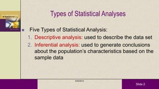
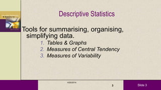
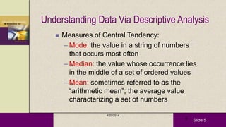
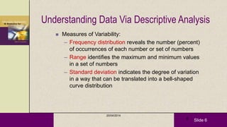
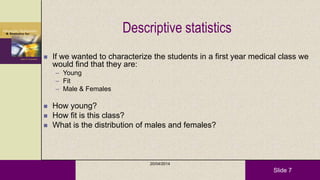
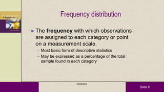
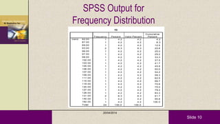
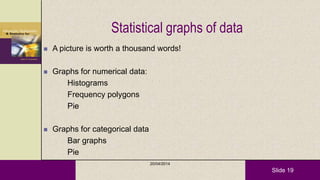
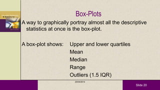
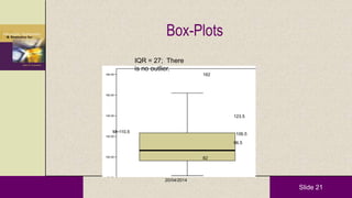
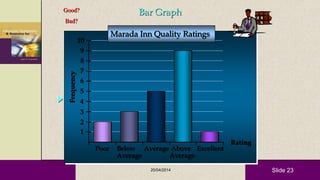
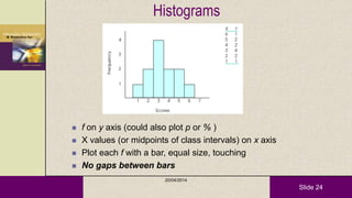
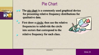
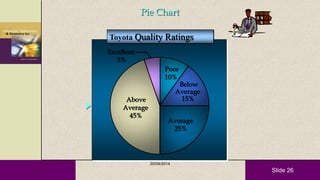
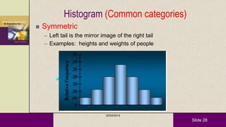
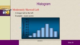
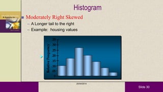
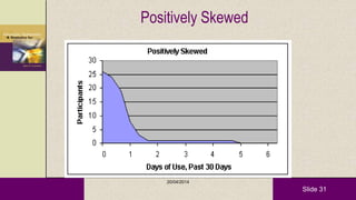
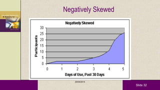
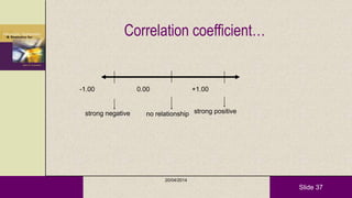
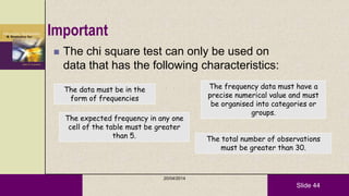
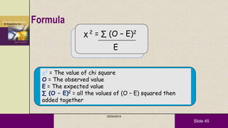
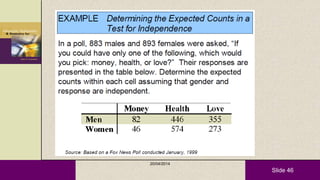
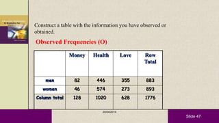
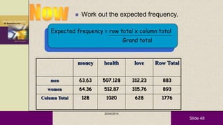
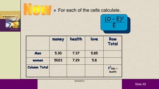
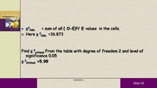
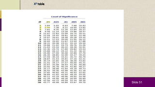
Slide 1
 Lecture by
 Dr Zahid Khan
 King Faisal University,KSA.
1
Descriptive Statistics
Slide 2
4/20/2014
2
Types of Statistical Analyses
 Five Types of Statistical Analysis:
1. Descriptive analysis: used to describe the data set
2. Inferential analysis: used to generate conclusions
about the population’s characteristics based on the
sample data
Slide 3
Descriptive Statistics
Tools for summarising, organising,
simplifying data.
1. Tables & Graphs
2. Measures of Central Tendency
3. Measures of Variability
4/20/2014
3
Slide 4
4/20/2014
4
Understanding Data Via Descriptive Analysis
 Two sets of descriptive measures:
–Measures of central tendency: used to report a
single piece of information that describes the most
typical response to a question
–Measures of variability: used to reveal the typical
difference between the values in a set of values
Slide 5
4/20/2014
5
Understanding Data Via Descriptive Analysis
 Measures of Central Tendency:
– Mode: the value in a string of numbers
that occurs most often
– Median: the value whose occurrence lies
in the middle of a set of ordered values
– Mean: sometimes referred to as the
―arithmetic mean‖; the average value
characterizing a set of numbers
Slide 6
20/04/2014
6
Understanding Data Via Descriptive Analysis
 Measures of Variability:
– Frequency distribution reveals the number (percent)
of occurrences of each number or set of numbers
– Range identifies the maximum and minimum values
in a set of numbers
– Standard deviation indicates the degree of variation
in a way that can be translated into a bell-shaped
curve distribution
Slide 7
Descriptive statistics
 If we wanted to characterize the students in a first year medical class we
would find that they are:
– Young
– Fit
– Male & Females
 How young?
 How fit is this class?
 What is the distribution of males and females?
20/04/2014
Slide 8
Frequency distribution
 The frequency with which observations
are assigned to each category or point
on a measurement scale.
– Most basic form of descriptive statistics
– May be expressed as a percentage of the total
sample found in each category
20/04/2014
Slide 9
Frequency distribution
 The distribution is ―read‖ differently depending upon
the measurement level
– Nominal scales are read as discrete measurements at each level
– Ordinal measures show tendencies, but categories should not be
compared
– Interval and ratio scales allow for comparison among categories
20/04/2014
Slide 10
SPSS Output for
Frequency Distribution
IQ
1 4.2 4.2 4.2
1 4.2 4.2 8.3
1 4.2 4.2 12.5
2 8.3 8.3 20.8
1 4.2 4.2 25.0
1 4.2 4.2 29.2
1 4.2 4.2 33.3
1 4.2 4.2 37.5
1 4.2 4.2 41.7
1 4.2 4.2 45.8
1 4.2 4.2 50.0
1 4.2 4.2 54.2
1 4.2 4.2 58.3
1 4.2 4.2 62.5
1 4.2 4.2 66.7
1 4.2 4.2 70.8
1 4.2 4.2 75.0
1 4.2 4.2 79.2
1 4.2 4.2 83.3
2 8.3 8.3 91.7
1 4.2 4.2 95.8
1 4.2 4.2 100.0
24 100.0 100.0
82.00
87.00
89.00
93.00
96.00
97.00
98.00
102.00
103.00
105.00
106.00
107.00
109.00
111.00
115.00
119.00
120.00
127.00
128.00
131.00
140.00
162.00
Total
Valid
Frequency Percent Valid Percent
Cumulative
Percent
20/04/2014
Slide 11
Grouped Relative Frequency Distribution
Relative Frequency Distribution of IQ for Two Classes
IQ FrequencyPercent Cumulative Percent
80 – 89 3 12.5 12.5
90 – 99 5 20.8 33.3
100 – 109 6 25.0 58.3
110 – 119 3 12.5 70.8
120 – 129 3 12.5 83.3
130 – 139 2 8.3 91.6
140 – 149 1 4.2 95.8
150 and over 1 4.2 100.0
Total 24 100.0 100.0
20/04/2014
Slide 12
Discrete and Continuous data
 Data consisting of numerical (quantitative) variables can be further
divided into two groups: discrete and continuous.
1. If the set of all possible values, when pictured on the number line,
consists only of isolated points.
2. If the set of all values, when pictured on the number line, consists of
intervals.
 The most common type of discrete variable we will encounter is a
counting variable.
20/04/2014
Slide 13
Accuracy & Precision
 Accuracy: the closeness of the measurements to the “actual” or “real” value
of the physical quantity.
– Statistically this is estimated using the standard error of the mean
 Precision: is used to indicate the closeness with which the measurements
agree with one another.
- Statistically the precision is estimated by the standard deviation of the
mean
Precision is related to random errors that can be dealt with using
statistics
Accuracy is related to systematic errors and are difficult to deal with
using statistics
20/04/2014
Slide 14
Accuracy and precision:
The target analogy
High accuracy but
low precision
High precision but
low accuracy
What does High accuracy and high precision look like?
20/04/2014
Slide 15
Accuracy and precision:
The target analogy
High accuracy and high precision
20/04/2014
Slide 16
Two types of error
 Systematic error
– Poor accuracy
– Definite causes
– Reproducible
 Random error
– Poor precision
– Non-specific causes
– Not reproducible
20/04/2014
Slide 17
Systematic error
 Diagnosis
– Errors have consistent signs
– Errors have consistent magnitude
 Treatment
– Calibration
– Correcting procedural flaws
– Checking with a different procedure
20/04/2014
Slide 18
Random error
 Diagnosis
– Errors have random sign
– Small errors more likely than large errors
 Treatment
– Take more measurements
– Improve technique
– Higher instrumental precision
20/04/2014
Slide 19
Statistical graphs of data
 A picture is worth a thousand words!
 Graphs for numerical data:
Histograms
Frequency polygons
Pie
 Graphs for categorical data
Bar graphs
Pie
20/04/2014
Slide 20
Box-Plots
A way to graphically portray almost all the descriptive
statistics at once is the box-plot.
A box-plot shows: Upper and lower quartiles
Mean
Median
Range
Outliers (1.5 IQR)
20/04/2014
Slide 21
Box-Plots
IQ
80.00
100.00
120.00
140.00
160.00
180.00
123.5
96.5
106.5
82
162
M=110.5
IQR = 27; There
is no outlier.
20/04/2014
Slide 22
Bar Graphs
 For categorical data
 Like a histogram, but with gaps between bars to show
that each bar is a separate group.
 Useful for showing two samples side-by-side
20/04/2014
Slide 23
Poor Below
Average
Average Above
Average
Excellent
Frequency
Rating
Bar Graph
1
2
3
4
5
6
7
8
9
10
Marada Inn Quality Ratings
Good?
Bad?
20/04/2014
Slide 24
Histograms
 f on y axis (could also plot p or % )
 X values (or midpoints of class intervals) on x axis
 Plot each f with a bar, equal size, touching
 No gaps between bars
20/04/2014
Slide 25
Pie Chart
 The pie chart is a commonly used graphical device
for presenting relative frequency distributions for
qualitative data.
 First draw a circle; then use the relative
frequencies to subdivide the circle
into sectors that correspond to the
relative frequency for each class.
20/04/2014
Slide 26
Below
Average
15%
Average
25%
Above
Average
45%
Poor
10%
Excellent
5%
Toyota Quality Ratings
Pie Chart
20/04/2014
Slide 27
Skewness of distributions
 Measures look at how lopsided distributions are—how far from the ideal
of the normal curve they are
 When the median and the mean are different, the distribution is skewed.
The greater the difference, the greater the skew.
 Distributions that trail away to the left are negatively skewed and those
that trail away to the right are positively skewed
 If the skewness is extreme, the researcher should either transform the
data to make them better resemble a normal curve or else use a
different set of statistics—nonparametric statistics—to carry out the
analysis
20/04/2014
Slide 28
 Symmetric
– Left tail is the mirror image of the right tail
– Examples: heights and weights of people
Histogram (Common categories)
RelativeFrequency
.05
.10
.15
.20
.25
.30
.35
0
20/04/2014
Slide 29
Histogram
 Moderately Skewed Left
– A longer tail to the left
– Example: exam scores
RelativeFrequency
.05
.10
.15
.20
.25
.30
.35
0
20/04/2014
Slide 30
 Moderately Right Skewed
– A Longer tail to the right
– Example: housing values
Histogram
RelativeFrequency
.05
.10
.15
.20
.25
.30
.35
0
20/04/2014
Slide 31
Positively Skewed
20/04/2014
Slide 32
Negatively Skewed
20/04/2014
Slide 33
Symmetry: Kurtosis
 A high kurtosis distribution has a sharper "peak"
and fatter "tails", while a low kurtosis
distribution has a more rounded peak with wider
"shoulders".
20/04/2014
Slide 34
5. Measures of relationship…
 Spearman Rho
 Pearson r
20/04/2014
Slide 35
 correlations
 determines whether and to what degree a
relationship exists between two or more
quantifiable variables
 the degree of the relationship is expressed as a
coefficient of correlation.
 the presence of a correlation does not indicate
a cause-effect relationship primarily because of
the possibility of multiple confounding factors
20/04/2014
Slide 36
…the presence of a correlation does
not indicate a cause-effect
relationship primarily because of the
possibility of multiple confounding
factors
20/04/2014
Slide 37
Correlation coefficient…
-1.00 +1.00
strong negative strong positive
0.00
no relationship
20/04/2014
Slide 38
 Spearman Rho...
…a measure of correlation used for
rank and ordinal data
20/04/2014
Slide 39
 Pearson r...
…a measure of correlation used for
data of interval or ratio scales
…assumes that the relationship
between the variables being
correlated is linear
20/04/2014
Slide 40
So
 Descriptive statistics are used to summarize data from
individual respondents, etc.
– They help to make sense of large numbers of individual
responses, to communicate the essence of those responses to
others
 They focus on typical or average scores, the dispersion of
scores over the available responses, and the shape of the
response curve
20/04/2014
Slide 41
Chi square (χ2 ) test
20/04/2014
Slide 42
Used to:
 Test for goodness of fit
 Test for independence of attributes
 Testing homogeneity
 Testing given population variance
20/04/2014
Slide 43
Introduction
 The test we use to measure the differences between
what is observed and what is expected according to
an assumed hypothesis is called the chi-square test.
20/04/2014
Slide 44
Important
 The chi square test can only be used on
data that has the following characteristics:
The data must be in the
form of frequencies
The frequency data must have a
precise numerical value and must
be organised into categories or
groups.
The total number of observations
must be greater than 30.
The expected frequency in any one
cell of the table must be greater
than 5.
20/04/2014
Slide 45
Formula
χ 2 = ∑ (O – E)2
E
χ2 = The value of chi square
O = The observed value
E = The expected value
∑ (O – E)2 = all the values of (O – E) squared then
added together
20/04/2014
Slide 46
20/04/2014
Slide 47
Construct a table with the information you have observed or
obtained.
Observed Frequencies (O)
Money Health Love Row
Total
men 82 446 355 883
women 46 574 273 893
Column total 128 1020 628 1776
20/04/2014
Slide 48
 Work out the expected frequency.
Expected frequency = row total x column total
Grand total
money health love Row Total
men 63.63 507.128 312.23 883
women 64.36 512.87 315.76 893
Column Total 128 1020 628 1776
20/04/2014
Slide 49
 For each of the cells calculate.
money health love Row
Total
Men 5.30 7.37 5.85
women 5023 7.29 5.8
Column Total χ2
Calc. =
36.873
(O – E)2
E
20/04/2014
Slide 50
 χ2
Calc. = sum of all ( O-E)2/ E values in the cells.
 Here χ 2
Calc. =36.873
Find χ 2
critical From the table with degree of freedom 2 and level of
significance 0.05
χ 2
Critical =5.99
20/04/2014
Slide 51
Χ2 table
Slide 52
Conclusion
 Compare χ2
Calc. and Χ2
critical obtained from the table
 If χ2
Calc. Is larger than χ2
Critical. then reject null hypothesis and
accept the alternative
 Here since χ 2
Calc. is much greater than χ 2
Critical, we can easily
reject null hypothesis
that is ; there lies a relation between the gender and choice of
selection.
20/04/2014
Slide 53
Any Questions !!!!!
•Thank You.
53
20/04/2014

Descrptive statistics

  • 1.
    Slide 1  Lectureby  Dr Zahid Khan  King Faisal University,KSA. 1 Descriptive Statistics
  • 2.
    Slide 2 4/20/2014 2 Types ofStatistical Analyses  Five Types of Statistical Analysis: 1. Descriptive analysis: used to describe the data set 2. Inferential analysis: used to generate conclusions about the population’s characteristics based on the sample data
  • 3.
    Slide 3 Descriptive Statistics Toolsfor summarising, organising, simplifying data. 1. Tables & Graphs 2. Measures of Central Tendency 3. Measures of Variability 4/20/2014 3
  • 4.
    Slide 4 4/20/2014 4 Understanding DataVia Descriptive Analysis  Two sets of descriptive measures: –Measures of central tendency: used to report a single piece of information that describes the most typical response to a question –Measures of variability: used to reveal the typical difference between the values in a set of values
  • 5.
    Slide 5 4/20/2014 5 Understanding DataVia Descriptive Analysis  Measures of Central Tendency: – Mode: the value in a string of numbers that occurs most often – Median: the value whose occurrence lies in the middle of a set of ordered values – Mean: sometimes referred to as the ―arithmetic mean‖; the average value characterizing a set of numbers
  • 6.
    Slide 6 20/04/2014 6 Understanding DataVia Descriptive Analysis  Measures of Variability: – Frequency distribution reveals the number (percent) of occurrences of each number or set of numbers – Range identifies the maximum and minimum values in a set of numbers – Standard deviation indicates the degree of variation in a way that can be translated into a bell-shaped curve distribution
  • 7.
    Slide 7 Descriptive statistics If we wanted to characterize the students in a first year medical class we would find that they are: – Young – Fit – Male & Females  How young?  How fit is this class?  What is the distribution of males and females? 20/04/2014
  • 8.
    Slide 8 Frequency distribution The frequency with which observations are assigned to each category or point on a measurement scale. – Most basic form of descriptive statistics – May be expressed as a percentage of the total sample found in each category 20/04/2014
  • 9.
    Slide 9 Frequency distribution The distribution is ―read‖ differently depending upon the measurement level – Nominal scales are read as discrete measurements at each level – Ordinal measures show tendencies, but categories should not be compared – Interval and ratio scales allow for comparison among categories 20/04/2014
  • 10.
    Slide 10 SPSS Outputfor Frequency Distribution IQ 1 4.2 4.2 4.2 1 4.2 4.2 8.3 1 4.2 4.2 12.5 2 8.3 8.3 20.8 1 4.2 4.2 25.0 1 4.2 4.2 29.2 1 4.2 4.2 33.3 1 4.2 4.2 37.5 1 4.2 4.2 41.7 1 4.2 4.2 45.8 1 4.2 4.2 50.0 1 4.2 4.2 54.2 1 4.2 4.2 58.3 1 4.2 4.2 62.5 1 4.2 4.2 66.7 1 4.2 4.2 70.8 1 4.2 4.2 75.0 1 4.2 4.2 79.2 1 4.2 4.2 83.3 2 8.3 8.3 91.7 1 4.2 4.2 95.8 1 4.2 4.2 100.0 24 100.0 100.0 82.00 87.00 89.00 93.00 96.00 97.00 98.00 102.00 103.00 105.00 106.00 107.00 109.00 111.00 115.00 119.00 120.00 127.00 128.00 131.00 140.00 162.00 Total Valid Frequency Percent Valid Percent Cumulative Percent 20/04/2014
  • 11.
    Slide 11 Grouped RelativeFrequency Distribution Relative Frequency Distribution of IQ for Two Classes IQ FrequencyPercent Cumulative Percent 80 – 89 3 12.5 12.5 90 – 99 5 20.8 33.3 100 – 109 6 25.0 58.3 110 – 119 3 12.5 70.8 120 – 129 3 12.5 83.3 130 – 139 2 8.3 91.6 140 – 149 1 4.2 95.8 150 and over 1 4.2 100.0 Total 24 100.0 100.0 20/04/2014
  • 12.
    Slide 12 Discrete andContinuous data  Data consisting of numerical (quantitative) variables can be further divided into two groups: discrete and continuous. 1. If the set of all possible values, when pictured on the number line, consists only of isolated points. 2. If the set of all values, when pictured on the number line, consists of intervals.  The most common type of discrete variable we will encounter is a counting variable. 20/04/2014
  • 13.
    Slide 13 Accuracy &Precision  Accuracy: the closeness of the measurements to the “actual” or “real” value of the physical quantity. – Statistically this is estimated using the standard error of the mean  Precision: is used to indicate the closeness with which the measurements agree with one another. - Statistically the precision is estimated by the standard deviation of the mean Precision is related to random errors that can be dealt with using statistics Accuracy is related to systematic errors and are difficult to deal with using statistics 20/04/2014
  • 14.
    Slide 14 Accuracy andprecision: The target analogy High accuracy but low precision High precision but low accuracy What does High accuracy and high precision look like? 20/04/2014
  • 15.
    Slide 15 Accuracy andprecision: The target analogy High accuracy and high precision 20/04/2014
  • 16.
    Slide 16 Two typesof error  Systematic error – Poor accuracy – Definite causes – Reproducible  Random error – Poor precision – Non-specific causes – Not reproducible 20/04/2014
  • 17.
    Slide 17 Systematic error Diagnosis – Errors have consistent signs – Errors have consistent magnitude  Treatment – Calibration – Correcting procedural flaws – Checking with a different procedure 20/04/2014
  • 18.
    Slide 18 Random error Diagnosis – Errors have random sign – Small errors more likely than large errors  Treatment – Take more measurements – Improve technique – Higher instrumental precision 20/04/2014
  • 19.
    Slide 19 Statistical graphsof data  A picture is worth a thousand words!  Graphs for numerical data: Histograms Frequency polygons Pie  Graphs for categorical data Bar graphs Pie 20/04/2014
  • 20.
    Slide 20 Box-Plots A wayto graphically portray almost all the descriptive statistics at once is the box-plot. A box-plot shows: Upper and lower quartiles Mean Median Range Outliers (1.5 IQR) 20/04/2014
  • 21.
  • 22.
    Slide 22 Bar Graphs For categorical data  Like a histogram, but with gaps between bars to show that each bar is a separate group.  Useful for showing two samples side-by-side 20/04/2014
  • 23.
    Slide 23 Poor Below Average AverageAbove Average Excellent Frequency Rating Bar Graph 1 2 3 4 5 6 7 8 9 10 Marada Inn Quality Ratings Good? Bad? 20/04/2014
  • 24.
    Slide 24 Histograms  fon y axis (could also plot p or % )  X values (or midpoints of class intervals) on x axis  Plot each f with a bar, equal size, touching  No gaps between bars 20/04/2014
  • 25.
    Slide 25 Pie Chart The pie chart is a commonly used graphical device for presenting relative frequency distributions for qualitative data.  First draw a circle; then use the relative frequencies to subdivide the circle into sectors that correspond to the relative frequency for each class. 20/04/2014
  • 26.
  • 27.
    Slide 27 Skewness ofdistributions  Measures look at how lopsided distributions are—how far from the ideal of the normal curve they are  When the median and the mean are different, the distribution is skewed. The greater the difference, the greater the skew.  Distributions that trail away to the left are negatively skewed and those that trail away to the right are positively skewed  If the skewness is extreme, the researcher should either transform the data to make them better resemble a normal curve or else use a different set of statistics—nonparametric statistics—to carry out the analysis 20/04/2014
  • 28.
    Slide 28  Symmetric –Left tail is the mirror image of the right tail – Examples: heights and weights of people Histogram (Common categories) RelativeFrequency .05 .10 .15 .20 .25 .30 .35 0 20/04/2014
  • 29.
    Slide 29 Histogram  ModeratelySkewed Left – A longer tail to the left – Example: exam scores RelativeFrequency .05 .10 .15 .20 .25 .30 .35 0 20/04/2014
  • 30.
    Slide 30  ModeratelyRight Skewed – A Longer tail to the right – Example: housing values Histogram RelativeFrequency .05 .10 .15 .20 .25 .30 .35 0 20/04/2014
  • 31.
  • 32.
  • 33.
    Slide 33 Symmetry: Kurtosis A high kurtosis distribution has a sharper "peak" and fatter "tails", while a low kurtosis distribution has a more rounded peak with wider "shoulders". 20/04/2014
  • 34.
    Slide 34 5. Measuresof relationship…  Spearman Rho  Pearson r 20/04/2014
  • 35.
    Slide 35  correlations determines whether and to what degree a relationship exists between two or more quantifiable variables  the degree of the relationship is expressed as a coefficient of correlation.  the presence of a correlation does not indicate a cause-effect relationship primarily because of the possibility of multiple confounding factors 20/04/2014
  • 36.
    Slide 36 …the presenceof a correlation does not indicate a cause-effect relationship primarily because of the possibility of multiple confounding factors 20/04/2014
  • 37.
    Slide 37 Correlation coefficient… -1.00+1.00 strong negative strong positive 0.00 no relationship 20/04/2014
  • 38.
    Slide 38  SpearmanRho... …a measure of correlation used for rank and ordinal data 20/04/2014
  • 39.
    Slide 39  Pearsonr... …a measure of correlation used for data of interval or ratio scales …assumes that the relationship between the variables being correlated is linear 20/04/2014
  • 40.
    Slide 40 So  Descriptivestatistics are used to summarize data from individual respondents, etc. – They help to make sense of large numbers of individual responses, to communicate the essence of those responses to others  They focus on typical or average scores, the dispersion of scores over the available responses, and the shape of the response curve 20/04/2014
  • 41.
    Slide 41 Chi square(χ2 ) test 20/04/2014
  • 42.
    Slide 42 Used to: Test for goodness of fit  Test for independence of attributes  Testing homogeneity  Testing given population variance 20/04/2014
  • 43.
    Slide 43 Introduction  Thetest we use to measure the differences between what is observed and what is expected according to an assumed hypothesis is called the chi-square test. 20/04/2014
  • 44.
    Slide 44 Important  Thechi square test can only be used on data that has the following characteristics: The data must be in the form of frequencies The frequency data must have a precise numerical value and must be organised into categories or groups. The total number of observations must be greater than 30. The expected frequency in any one cell of the table must be greater than 5. 20/04/2014
  • 45.
    Slide 45 Formula χ 2= ∑ (O – E)2 E χ2 = The value of chi square O = The observed value E = The expected value ∑ (O – E)2 = all the values of (O – E) squared then added together 20/04/2014
  • 46.
  • 47.
    Slide 47 Construct atable with the information you have observed or obtained. Observed Frequencies (O) Money Health Love Row Total men 82 446 355 883 women 46 574 273 893 Column total 128 1020 628 1776 20/04/2014
  • 48.
    Slide 48  Workout the expected frequency. Expected frequency = row total x column total Grand total money health love Row Total men 63.63 507.128 312.23 883 women 64.36 512.87 315.76 893 Column Total 128 1020 628 1776 20/04/2014
  • 49.
    Slide 49  Foreach of the cells calculate. money health love Row Total Men 5.30 7.37 5.85 women 5023 7.29 5.8 Column Total χ2 Calc. = 36.873 (O – E)2 E 20/04/2014
  • 50.
    Slide 50  χ2 Calc.= sum of all ( O-E)2/ E values in the cells.  Here χ 2 Calc. =36.873 Find χ 2 critical From the table with degree of freedom 2 and level of significance 0.05 χ 2 Critical =5.99 20/04/2014
  • 51.
  • 52.
    Slide 52 Conclusion  Compareχ2 Calc. and Χ2 critical obtained from the table  If χ2 Calc. Is larger than χ2 Critical. then reject null hypothesis and accept the alternative  Here since χ 2 Calc. is much greater than χ 2 Critical, we can easily reject null hypothesis that is ; there lies a relation between the gender and choice of selection. 20/04/2014
  • 53.
    Slide 53 Any Questions!!!!! •Thank You. 53 20/04/2014