The document provides an overview of statistics, including its definition as the science of collecting, analyzing, and interpreting data for improved decision-making. It covers types of statistics such as descriptive and inferential, along with methods of sampling, data collection, and presentation techniques like histograms and pie charts. Additionally, it distinguishes between qualitative and quantitative data and details their respective subcategories and measurement scales.

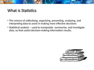
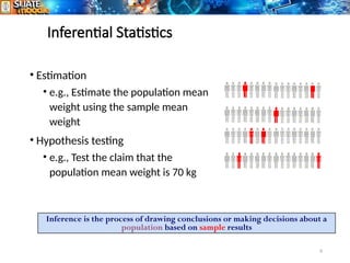
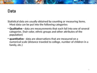
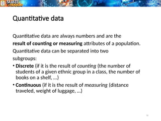
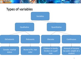
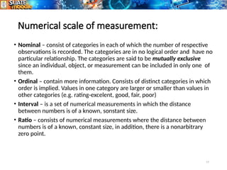
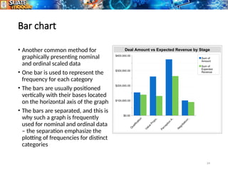
1. 1
HNDIT 1214
Statistics for IT
1. Introduction To Statistics

2. 2

3. 3
What is Statistics
• The science of collectiong, organizing, presenting, analyzing, and
interpreting data to assist in making more effective decisions
• Statistical analysis – used to manipulate summarize, and investigate
data, so that useful decision-making information results.

4. 4
Types of statistics
• Descriptive statistics – Methods of organizing, summarizing, and
presenting data in an informative way
• Inferential statistics – The methods used to determine something
about a population on the basis of a sample
• Population –The entire set of individuals or objects of interest or the
measurements obtained from all individuals or objects of interest
• Sample – A portion, or part, of the population of interest

5. 5

6. 6
Inferential Statistics
• Estimation
• e.g., Estimate the population mean
weight using the sample mean
weight
• Hypothesis testing
• e.g., Test the claim that the
population mean weight is 70 kg
Inference is the process of drawing conclusions or making decisions about a
population based on sample results

7. 7
Sampling
a sample should have the same characteristics
as the population it is representing.
Sampling can be:
• with replacement: a member of the population may be chosen more
than once (picking the candy from the bowl)
• without replacement: a member of the population may be chosen
only once (lottery ticket)

8. 8
Sampling methods
Sampling methods can be:
• random (each member of the population has an equal chance
of being selected)
• nonrandom
The actual process of sampling causes sampling
errors. For example, the sample may not be large
enough or representative of the population. Factors not
related to the sampling process cause nonsampling
errors. A defective counting device can cause a
nonsampling error.

9. 9
Random sampling methods
• Simple random sample (each sample of the same size has
an equal chance of being selected)
• Stratified sample (divide the population into groups called
strata and then take a sample from each stratum)
• Cluster sample (divide the population into strata and then
randomly select some of the strata. All the members from
these strata are in the cluster sample.)
• Systematic sample (randomly select a starting point and
take every n-th piece of data from a listing of the population)

10. 10
Descriptive Statistics
•Collect data
•e.g., Survey
•Present data
•e.g., Tables and graphs
•Summarize data
•e.g., Sample mean = i
X
n


11. 11
Statistical data
 The collection of data that are relevant to the problem being studied
is commonly the most difficult, expensive, and time-consuming part
of the entire research project.
 Statistical data are usually obtained by counting or measuring items.
 Primary data are collected specifically for the analysis desired
 Secondary data have already been compiled and are available for statistical
analysis
 A variable is an item of interest that can take on many different
numerical values.
 A constant has a fixed numerical value.

12. 12
Data Collection Methods
• Data can be collected in a variety of ways
• Interviews
• Face -to -face interviews
• Telephone interviews
• Computer Assisted Personal Interviewing (CAPI)
• Questionnaires
• Paper-pencil-questionnaires
• Web based questionnaires
• Survey
• Observation
• Exercise : Discuss advantage and disadvantage of each above data
collective methods

13. 13
Data
Statistical data are usually obtained by counting or measuring items.
Most data can be put into the following categories:
• Qualitative - data are measurements that each fail into one of several
categories. (hair color, ethnic groups and other attributes of the
population)
• quantitative - data are observations that are measured on a
numerical scale (distance traveled to college, number of children in a
family, etc.)

14. 14
Qualitative data
Qualitative data are generally described by words or
letters. They are not as widely used as quantitative data
because many numerical techniques do not apply to the
qualitative data. For example, it does not make sense to
find an average hair color or blood type.
Qualitative data can be separated into two subgroups:
 Dichotomic (if it takes the form of a word with two options
(gender - male or female)
 Polynomic (if it takes the form of a word with more than
two options (education - primary school, secondary school
and university).

15. 15
Quantitative data
Quantitative data are always numbers and are the
result of counting or measuring attributes of a population.
Quantitative data can be separated into two
subgroups:
• Discrete (if it is the result of counting (the number of
students of a given ethnic group in a class, the number of
books on a shelf, ...)
• Continuous (if it is the result of measuring (distance
traveled, weight of luggage, …)

16. 16
Types of variables
Variables
Quantitative
Qualitative
Dichotomic Polynomic Discrete Continuous
Gender, marital
status
Brand of Pc, hair
color
Children in family,
Strokes on a golf
hole
Amount of income
tax paid, weight of a
student

17. 17
Numerical scale of measurement:
• Nominal – consist of categories in each of which the number of respective
observations is recorded. The categories are in no logical order and have no
particular relationship. The categories are said to be mutually exclusive
since an individual, object, or measurement can be included in only one of
them.
• Ordinal – contain more information. Consists of distinct categories in which
order is implied. Values in one category are larger or smaller than values in
other categories (e.g. rating-excelent, good, fair, poor)
• Interval – is a set of numerical measurements in which the distance
between numbers is of a known, sonstant size.
• Ratio – consists of numerical measurements where the distance between
numbers is of a known, constant size, in addition, there is a nonarbitrary
zero point.

18. 18

19. 19
Data presentation
„ The question is“ said Alice, „whether you can
make words mean so many different things.“
„The question is,“ said Humpty Dumpty, „which is
to be master-that´s all.“ (Lewis Carroll)

20. 20
Histogram
• Frequently used to graphically
present interval and ratio data
• Is often used for interval and
ratio data
• The adjacent bars indicate that a
numerical range is being
summarized by indicating the
frequencies in arbitrarily chosen
classes

21. 21
Frequency polygon
• Another common method for
graphically presenting interval
and ratio data
• To construct a frequency
polygon mark the frequencies
on the vertical axis and the
values of the variable being
measured on the horizontal axis,
as with the histogram.
• If the purpose of presenting is
comparation with other
distributions, the frequency
polygon provides a good
summary of the data

22. 22
Ogive
• A graph of a cumulative
frequency distribution
• Ogive is used when one wants to
determine how many
observations lie above or below
a certain value in a distribution.
• First cumulative frequency
distribution is constructed
• Cumulative frequencies are
plotted at the upper class limit of
each category
• Ogive can also be constructed for
a relative frequency distribution.

23. 23
Pie Chart
• The pie chart is an effective way
of displaying the percentage
breakdown of data by category.
• Useful if the relative sizes of the
data components are to be
emphasized
• Pie charts also provide an
effective way of presenting
ratio- or interval-scaled data
after they have been organized
into categories

24. 24
Bar chart
• Another common method for
graphically presenting nominal
and ordinal scaled data
• One bar is used to represent the
frequency for each category
• The bars are usually positioned
vertically with their bases located
on the horizontal axis of the graph
• The bars are separated, and this is
why such a graph is frequently
used for nominal and ordinal data
– the separation emphasize the
plotting of frequencies for distinct
categories

25. 25
Time Series Graph
•The time series graph is
a graph of data that
have been measured
over time.
•The horizontal axis of
this graph represents
time periods and the
vertical axis shows the
numerical values
corresponding to these
time periods

26. 26