Statistics is the science of data, but in reality statistics is both the science and the art of collecting, organizing, summarizing, analyzing and drawing conclusion based on data.
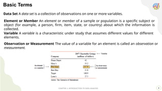
Population or Target Population A population consists of all elements—individuals, items, or objects—whose characteristics are being studied. The population that is being studied is also called the target population.


![CHAPTER 1: INTRODUCTION TO DATA ANALYSIS 22
i. Mean:
Example of Measures of Central Tendency (Ungrouped Data)
The data represent the number of days off per year for a sample of individuals selected from nine different
countries. Find the mean, median and mode.
20, 26, 40, 36, 23, 42, 35, 24, 30
Solution:
ii. Median:
Step 1: 20, 23, 24, 26, 30, 35, 36, 40, 42
Step 2: [(n+1)/2]th = 5th
Median = 30
iii. Mode for ungrouped
• No Mode for this dataset](https://image.slidesharecdn.com/introductiontodataanalysispart1-250918034525-4f6146f7/85/Introduction_to_Data_Analysis_Part_1-pptx-22-320.jpg)