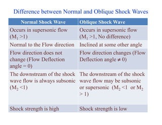
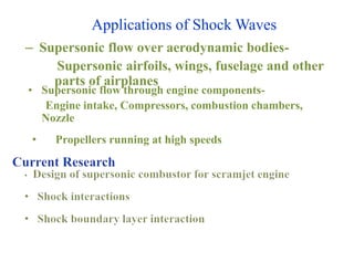
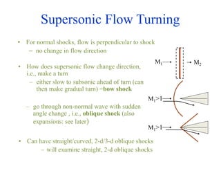
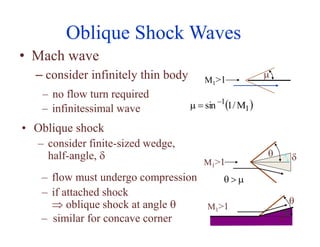
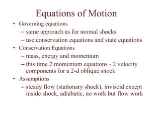
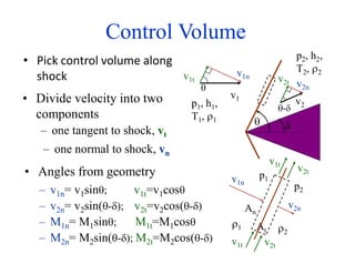
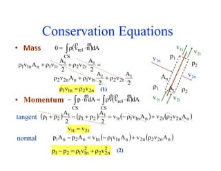
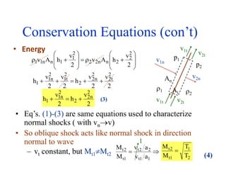
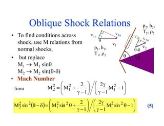
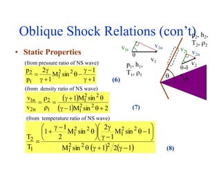
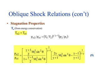
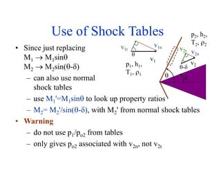
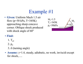
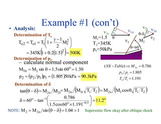
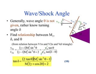
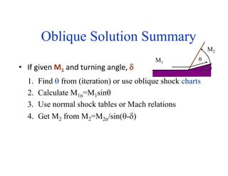
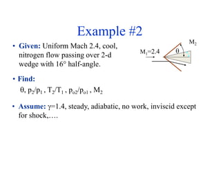
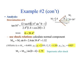
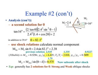
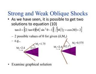
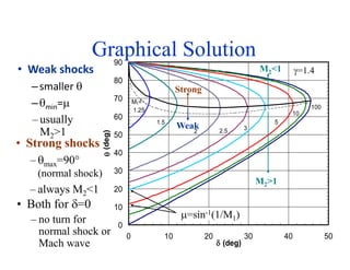
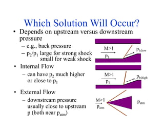
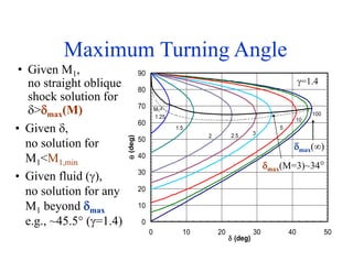
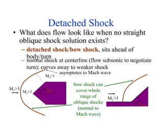
This document discusses oblique shock waves that occur in supersonic flows when the flow direction changes. It provides the governing equations for analyzing oblique shock waves using conservation of mass, momentum, and energy across a control volume. The equations show that an oblique shock acts like a normal shock in the direction normal to the wave. Relations are developed to determine the post-shock Mach number, static properties, and stagnation properties in terms of the shock angle and pre-shock Mach number using normal shock tables. An example problem applies these relations to analyze an oblique shock occurring at a sharp concave corner.

1. ME 6604 – GAS DYNAMICS AND JET PROPULSION
UNIT – III SHOCK WAVES
Mrs. N. PREMALATHA
ASSOCIATE PROFESSOR
DEPARTMENT OF MECHANICAL ENGG

2. Significance of Compressible Flows
• Isentropic Flow
a. Entropy remains constant
b. All the stagnation parameters remain constant
• Fanno Flow
a. Entropy changes (Non-isentropic process)
b. Stagnation temperature remains constant
• Rayleigh Flow
a. Entropy changes (Non-isentropic process)
b. Stagnation temperature changes
• Flow Through Shock Waves
a. Entropy increases (Non-isentropic process)
b. Stagnation temperature constant
Note: Isentropic flow tables are used for
All the flows. How?

3. Difference between Normal and Oblique Shock Waves
Normal Shock Wave Oblique Shock Wave
Occurs in supersonic flow
(M1 >1)
Occurs in supersonic flow
(M1 >1, No difference)
Normal to the Flow direction Inclined at some other angle
Flow direction does not
change (Flow Deflection
angle = 0)
Flow direction changes (Flow
Deflection angle  0)
The downstream of the shock
wave flow is always subsonic
(M2 <1)
The downstream of the shock
wave flow may be subsonic
or supersonic (M2 <1 or M2
> 1)
Shock strength is high Shock strength is low

4. Applications of Shock Waves
– Supersonic flow over aerodynamic bodies-
Supersonic airfoils, wings, fuselage and other
parts of airplanes
• Supersonic flow through engine components-
Engine intake, Compressors, combustion chambers,
Nozzle
• Propellers running at high speeds

5. Supersonic Flow Turning
• For normal shocks, flow is perpendicular to shock
– no change in flow direction
• How does supersonic flow change direction,
i.e., make a turn
– either slow to subsonic ahead of turn (can
then make gradual turn) =bow shock
M1 M2
M1>1
M1>1
– go through non-normal wave with sudden
angle change , i.e., oblique shock (also
expansions: see later)
• Can have straight/curved, 2-d/3-d oblique shocks
– will examine straight, 2-d oblique shocks

6. Oblique Shock Waves
• Mach wave
– consider infinitely thin body M1>1

• Oblique shock
– consider finite-sized wedge,
half-angle, 
M1>1

– no flow turn required

 1
1
M/1sin 
– infinitessimal wave

– flow must undergo compression
– if attached shock
 oblique shock at angle 
– similar for concave corner

M1>1


7. Equations of Motion
• Governing equations
– same approach as for normal shocks
– use conservation equations and state equations
• Conservation Equations
– mass, energy and momentum
– this time 2 momentum equations - 2 velocity
components for a 2-d oblique shock
• Assumptions
– steady flow (stationary shock), inviscid except
inside shock, adiabatic, no work but flow work

8. Control Volume
• Pick control volume along
shock
p1, h1,
T1, 1
v1
 
p2, h2,
T2, 2
v2

-
• Divide velocity into two
components
– one tangent to shock, vt
– one normal to shock, vn
• Angles from geometry
v1n
v2n
v1n
v2nAn
At
p1
p2
1 2
v1t v2t
v1t v2t
v1t
v2t
– v1n= v1sin; v1t=v1cos
– v2n= v2sin(-); v2t=v2cos(-)
– M1n= M1sin; M1t=M1cos
– M2n= M2sin(-); M2t=M2cos(-)

9. Conservation Equations
• Mass
v1n
v2nAn
At
p1
p2
1 2
v1t v2t
v1t
v2t
  Adnv0 rel
CS

 
2
A
v
2
A
vAv
2
A
v
2
A
vAv
t
t22
t
t11nn22
t
t22
t
t11nn11


• Momentum   
CS
rel
CS
AdnvvAdnp

tangent        nn22t2nn11t1
t
21
t
21 AvvAvv
2
A
pp
2
A
pp 
t2t1 vv 
normal    nn22n2nn11n1n2n1 AvvAvvApAp 
n22n11 vv  (1)
2
n22
2
n1121 vvpp  (2)

10. Conservation Equations (con’t)
• Energy
v1n
v2nAn
At
p1
p2
1 2
v1t v2t
v1t
v2t


















2
v
hAv
2
v
hAv
2
2
2nn22
2
1
1nn11
2
v
2
v
h
2
v
2
v
h
2
t2
2
n2
2
2
t1
2
n1
1 
2
v
h
2
v
h
2
n2
2
2
n1
1  (3)
• Eq’s. (1)-(3) are same equations used to characterize
normal shocks ( with vnv)
• So oblique shock acts like normal shock in direction
normal to wave
– vt constant, but Mt1Mt2 
11t
22t
1t
2t
av
av
M
M
(4)2
1
1t
2t
T
T
M
M

1

11. Oblique Shock Relations
• To find conditions across
shock, use M relations from
normal shocks,
• but replace
M1  M1 sin
M2  M2 sin(-)
• Mach Number
  1sinM
1
2
1
2
sinMsinM 22
1
22
1
22
2 
















1M
1
2
1
2
MM 2
1
2
1
2
2 















from
p1, h1,
T1, 1
v1
 
p2, h2,
T2, 2
v2

-
v1n
v2n
v1t v2t
(5)

12. Oblique Shock Relations (con’t)
• Static Properties
p1, h1,
T1, 1
v1
 
p2, h2,
T2, 2
v2

-
v1n
v2n
v1t v2t
(6)1
1
sinM
1
2
p
p 22
1
1
2






(from pressure ratio of NS wave)
(7)
 
  2sinM1
sinM1
v
v
22
1
22
1
1
2
n2
n1






(from density ratio of NS wave)
   121sinM
1sinM
1
2
sinM
2
1
1
T
T
222
1
22
1
22
1
1
2




















(8)
(from temperature ratio of NS wave)

13. Oblique Shock Relations (con’t)
• Stagnation Properties
1o2o TT 
To (from energy conservation)
   12
1
211o2o ppTTpp 































1
1
22
1
1
22
1
22
1
1o
2o
1
1
sinM
1
2
sinM
2
1
1
sinM
2
1
p
p
(9)

14. Use of Shock Tables
• Since just replacing
M1  M1sin
M2  M2sin(-)
– can also use normal
shock tables
– use M1'=M1sin to look up property ratios
– M2= M2'/sin(-), with M2' from normal shock tables
• Warning
– do not use p1/po2 from tables
– only gives po2 associated with v2n, not v2t
p1, h1,
T1, 1
v1
 
p2, h2,
T2, 2
v2

-
v1n
v2n
v1t v2t

15. Example #1
• Given: Uniform Mach 1.5 air
flow (p=50 kPa, T=345K)
approaching sharp concave
corner. Oblique shock produced
with shock angle of 60°
• Find:
1. To2
2. p2
3.  (turning angle)
• Assume: =1.4, steady, adiabatic, no work, inviscid except
for shock,….
=60°
M1=1.5
T1=345K
p1=50kPa

M2

16. Example #1 (con’t)• Analysis:
Determination of To
30.160sin5.1sinMM 1n1  
191.1
805.1
786.0)(
12
12
2



TT
pp
MTableNS n
– calculate normal component
   K5005.12.01K345
M
2
1
1TTT
2
2
111o2o






 

Determination of p2
    kPa3.90kPa50805.1pppp 1122 
Determination of 



2.11
191.160cos5.1
786.0
tan60 5.0
1







 

  t2n2 MMtan     211n221t1n2 TTcosMMTTMM 

v1t
v1
v1n
-
v2
v2n
v2t
  104.1sinMM n22 NOTE: Supersonic flow okay after oblique shock
=60°
M1=1.5
T1=345K
p1=50kPa

M2

17. Wave/Shock Angle
• Generally, wave angle  is not
given, rather know turning
angle 
• Find relationship between M1,
, and 
  
  22cosM
1sinMtan2
tan 2
1
22
1



 
v2
-
v2n
v1

v1nv1t
v2t
 
  2sinM1
sinM1
v
v
22
1
22
1
n2
n1



(from relation between V1n and V2n and Vel triangle)
 


tanv
tanv
t2
t1
1
(10)

18. Oblique Solution Summary
• If given M1 and turning angle, 
1. Find  from (iteration) or use oblique shock charts
2. Calculate M1n=M1sin
3. Use normal shock tables or Mach relations
4. Get M2 from M2=M2n/sin(-)
M1

M2

19. Example #2
• Given: Uniform Mach 2.4, cool,
nitrogen flow passing over 2-d
wedge with 16° half-angle.
• Find:
, p2/p1 , T2/T1 , po2/po1 , M2
• Assume: =1.4, steady, adiabatic, no work, inviscid except
for shock,….
M1=2.4 
M2

20. Example #2 (con’t)
• Analysis:
Determination of 
52.14.39sin4.2sinMM 1n1  
9227.0;335.1;535.2;6935.0)1.( 1212122  oon ppTTppMNSTable
– use shock relations calculate normal component
  75.1sinMM n22  Supersonic after shock
  
  22cos4.14.2
1sin4.2tan2
16tan 2
22



=16°M1=2.4 
M2
iterate 
4.39

21. Example #2 (con’t)
• Analysis (con’t):
38.21.82sin4.2sinMM 1n1  
5499.0;018.2;425.6;5256.0)( 1212122  oon ppTTppMNStable
– use shock relations calculate normal component
  575.0sinMM n22 
=16°M1=2.4 
M2
– a second solution for 
  
  22cos4.14.2
1sin4.2tan2
16tan 2
22



in addition to 39.4 
1.82
• Eqn generally has 2 solutions for : Strong and Weak oblique shocks
Now subsonic after shock
previous solution 2.535 1.335 0.9227
1.75

22. Strong and Weak Oblique Shocks
• As we have seen, it is possible to get two
solutions to equation (10)
– 2 possible values of  for given (,M1)
– e.g.,
      22cosM1sinMtan2tan 2
1
22
1 
M1=2.4 39.4°
M2=1.75
=16°
M1=2.4 82.1°
M2=0.575
=16°
• Examine graphical solution

23. Graphical Solution
• Weak shocks
–smaller 
–min=
0
10
20
30
40
50
60
70
80
90
0 10 20 30 40 50
 (deg)
(deg)
0
10
20
30
40
50
60
70
80
90
M1=
1.25
1.5
2 2.5 3
5
10
100
=1.4M2<1
M2>1
Strong
Weak
=sin-1(1/M1)
– usually
M2>1
• Strong shocks
– max=90°
(normal shock)
– always M2<1
• Both for =0
– no turn for
normal shock or
Mach wave

24. Which Solution Will Occur?
• Depends on upstream versus downstream
pressure
– e.g., back pressure
– p2/p1 large for strong shock
small for weak shock
• Internal Flow
– can have p2 much higher
or close to p1
M>1
p1
pb,high
M>1
p1
pb,low
• External Flow
– downstream pressure
usually close to upstream
p (both near patm)
M>1
patm
patm

25. Maximum Turning Angle
• Given M1,
no straight oblique
shock solution for
>max(M)
0
10
20
30
40
50
60
70
80
90
0 10 20 30 40 50
 (deg)
(deg)
0
10
20
30
40
50
60
70
80
90
M1=
1.25
1.5
2 2.5 3
5
10
100
=1.4
max(M=3)~34°
• Given ,
no solution for
M1<M1,min
• Given fluid (),
no solution for any
M1 beyond max
e.g., ~45.5° (=1.4)
max()

26. Detached Shock
• What does flow look like when no straight
oblique shock solution exists?
– detached shock/bow shock, sits ahead of
body/turn
M1>1
>max
bow shock can
cover whole
range of
oblique shocks
(normal to
Mach wave)
– normal shock at centerline (flow subsonic to negotiate
turn); curves away to weaker shock
asymptotes to Mach wave
M2<1
M2>1
M1>1 >ma
x

27. CRITICAL FLOW AND SHOCK WAVES
0.1 DivergenceDragCR MM
MCR
• Sharp increase in cd is combined effect of shock waves and flow separation
• Freestream Mach number at which cd begins to increase rapidly called Drag-
Divergence Mach number