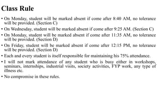
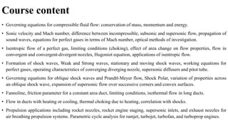
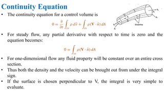
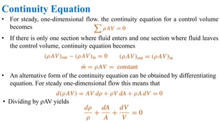
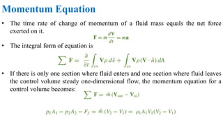
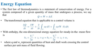
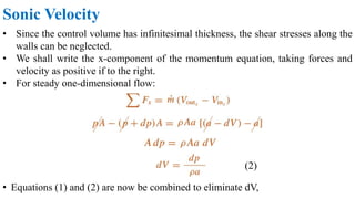
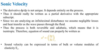
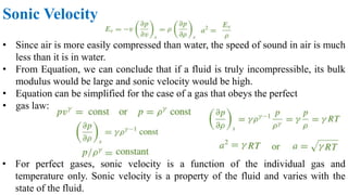
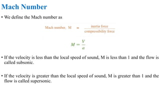
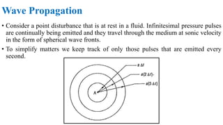
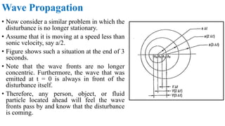
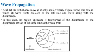
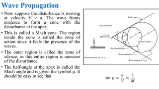
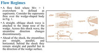
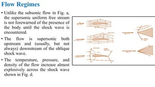
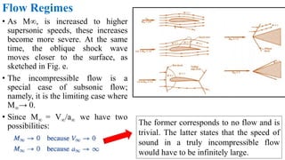
This document summarizes the key points from Week 1 of a course on compressible flows and propulsion systems. It outlines the class attendance rules, then provides an overview of the governing equations for compressible fluid flow and key terms like sonic velocity and Mach number. It also lists the course content, which will cover topics like isentropic flow, shock waves, and propulsion applications. The intended learning outcomes are also stated.

1. Lectures of Week 1
Introduction to Compressible Flows
Course Title: Compressible Flow and Propulsion System
Course Code: (ME-417)

2. Class Rule
• On Monday, student will be marked absent if come after 8:40 AM, no tolerance
will be provided. (Section C)
• On Wednesday, student will be marked absent if come after 9:25 AM. (Section C)
• On Monday, student will be marked absent if come after 11:35 AM, no tolerance
will be provided. (Section D)
• On Friday, student will be marked absent if come after 12:15 PM, no tolerance
will be provided. (Section D)
• Each and every student is itself responsible for maintaining his 75% attendance.
• I will not mark attendance of any student who is busy either in workshops,
seminars, internships, industrial visits, society activities, FYP work, any type of
illness etc.
• No compromise in these rules.

3. Course content
• Governing equations for compressible fluid flow: conservation of mass, momentum and energy.
• Sonic velocity and Mach number, difference between incompressible, subsonic and supersonic flow, propagation of
sound waves, equations for perfect gases in terms of Mach number, optical methods of investigation.
• Isentropic flow of a perfect gas, limiting conditions (choking), effect of area change on flow properties, flow in
convergent and convergent-divergent nozzles, Hugoniot equation, applications of isentropic flow.
• Formation of shock waves, Weak and Strong waves, stationary and moving shock waves, working equations for
perfect gases, operating characteristics of converging diverging nozzle, supersonic diffusers and pitot tube.
• Governing equations for oblique shock waves and Prandtl-Meyer flow, Shock Polar, variation of properties across
an oblique shock wave, expansion of supersonic flow over successive corners and convex surfaces.
• Fannoline, friction parameter for a constant area duct, limiting conditions, isothermal flow in long ducts.
• Flow in ducts with heating or cooling, thermal choking due to heating, correlation with shocks.
• Propulsion applications including rocket nozzles, rocket engine staging, supersonic inlets, and exhaust nozzles for
air breathing propulsion systems. Parametric cycle analysis for ramjet, turbojet, turbofan, and turboprop engines.

4. Course Learning Outcomes
No. CLO PLO
Taxonomy
Level
1
Explain different terms of compressible and isentropic
flows PLO – 1 C2
2
Solve cases of different non-isentropic flows such as
normal / oblique shock and flows with friction or heat
transfer
PLO – 2 C3
3
Analyze various shaft power and aircraft gas turbine
engines PLO – 3 C4
Test book: Gas Dynamics by M. Haluk Aksel

5. Compressible Flow and Propulsion System
Fluid flow with significant
density change
Introduction
A machine that produces thrust
to push an object forward
Gas dynamics Gas turbines

6. Compressible flow
• The course of compressible flow/gas dynamics is concerned with
the causes and the effects arising from the motion of
compressible fluids particularly gases.
• It is branch of more general subject of fluid dynamics.
• Compressible flow involves significant changes in density. It is
encountered in devices that involve the flow of gases at very high
speeds.
• Compressible flow combines fluid dynamics and
thermodynamics in that both are necessary to the development of
the required theoretical background.

7. Compressible flow
• The analysis of flow problems is based on the fundamental principles given
below:
1. Conservation of mass
2. Newton’s second law of motion
3. Conservation of energy

8. Continuity Equation
• For steady flow, any partial derivative with respect to time is zero and the
equation becomes:
• The continuity equation for a control volume is
• For one-dimensional flow any fluid property will be constant over an entire cross
section.
• Thus both the density and the velocity can be brought out from under the integral
sign.
• If the surface is chosen perpendicular to V, the integral is very simple to
evaluate.

9. Continuity Equation
• For steady, one-dimensional flow, the continuity equation for a control volume
becomes
• If there is only one section where fluid enters and one section where fluid leaves
the control volume, continuity equation becomes
• An alternative form of the continuity equation can be obtained by differentiating
equation. For steady one-dimensional flow this means that
• Dividing by ρAV yields

10. Momentum Equation
• The time rate of change of momentum of a fluid mass equals the net force
exerted on it.
• The integral form of equation is
• If there is only one section where fluid enters and one section where fluid leaves
the control volume steady one-dimensional flow, the momentum equation for a
control volume becomes:

11. Energy Equation
• The first law of thermodynamics is a statement of conservation of energy. For a
system composed of a given quantity of mass that undergoes a process, we say
that
• Thetransformed equation that is applicable to a control volume is
• With enthalpy, the one-dimensional energy equation for steady-in-the- mean flow
is
• where q and ws represent quantities of heat and shaft work crossing the control
surface per unit mass of fluid flowing.

12. Sonic Velocity
• A disturbance at a given point creates a region of
compressed molecules that is passed along to its
neighboring molecules and in so doing creates a
traveling wave.
• The speed at which this disturbance is propagated
through the medium is called the wave speed.
• This speed not only depends on the type of medium
and its thermodynamic state but is also a function
of the strength of the wave.
• The speed of waves of very small amplitude is
characteristic only of the medium and its state.
• Sound waves are infinitesimal waves (or weak
pressure pulses) which propagate at the
characteristic sonic velocity.

13. Sonic Velocity
• Consider a long constant-area tube filled with fluid and having a piston at one
end.
• The fluid is initially at rest. At a certain instant the piston is given an incremental
velocity dV to the left.
• The fluid particles immediately next to the piston are compressed a very small
amount as they acquire the velocity of the piston.
• As the piston (and these compressed particles) continue to move, the next group
of fluid particles is compressed.
• The wave front is observed to propagate through the fluid at the characteristic
sonic velocity of magnitude a.

14. Sonic Velocity
• All particles between the wave front and the piston are moving with velocity dV
to the left and have been compressed from ρ to ρ + dρ and have increased their
pressure from p to p + dp.
• For the analysis we choose the wave region as a control volume and assume the
wave front as a stationary wave.

15. • For an observer moving with this control volume, the fluid appears to enter the
control volume through surface area A with speed ‘a’ at pressure p and density ρ.
• The fluid leaves the control volume through surface area A with speed a –dV,
pressure p + dp and density ρ + dρ.
• When the continuity equation is applied to the flow through this control volume,
the result is
Sonic Velocity
(1)

16. Sonic Velocity
• Since the control volume has infinitesimal thickness, the shear stresses along the
walls can be neglected.
• We shall write the x-component of the momentum equation, taking forces and
velocity as positive if to the right.
• For steady one-dimensional flow:
(2)
• Equations (1) and (2) are now be combined to eliminate dV,

17. Sonic Velocity
• The derivative dp/dρ is not unique. It depends entirely on the process.
• Thus it should really be written as a partial derivative with the appropriate
subscript.
• Since we are analyzing an infinitesimal disturbance we assume negligible losses
and heat transfer as the wave passes through the fluid.
• Thus the process is both reversible and adiabatic, which means that it is
isentropic. Therefore, equation of sound can properly be written as
• Sound velocity can be expressed in terms of bulk or volume modulus of
elasticity Ev.

18. Sonic Velocity
• Since air is more easily compressed than water, the speed of sound in air is much
less than it is in water.
• From Equation, we can conclude that if a fluid is truly incompressible, its bulk
modulus would be large and sonic velocity would be high.
• Equation can be simplified for the case of a gas that obeys the perfect
• gas law:
• For perfect gases, sonic velocity is a function of the individual gas and
temperature only. Sonic velocity is a property of the fluid and varies with the
state of the fluid.

19. Mach Number
• We define the Mach number as
• If the velocity is less than the local speed of sound, M is less than 1 and the flow is
called subsonic.
• If the velocity is greater than the local speed of sound, M is greater than 1 and the
flow is called supersonic.

20. Wave Propagation
• Consider a point disturbance that is at rest in a fluid. Infinitesimal pressure pulses
are continually being emitted and they travel through the medium at sonic velocity
in the form of spherical wave fronts.
• To simplify matters we keep track of only those pulses that are emitted every
second.

21. • Now consider a similar problem in which the
disturbance is no longer stationary.
• Assume that it is moving at a speed less than
sonic velocity, say a/2.
• Figure shows such a situation at the end of 3
seconds.
• Note that the wave fronts are no longer
concentric. Furthermore, the wave that was
emitted at t = 0 is always in front of the
disturbance itself.
• Therefore, any person, object, or fluid
particle located ahead will feel the wave
fronts pass by and know that the disturbance
is coming.
Wave Propagation

22. • Next, let the disturbance move at exactly sonic velocity. Figure shows this case in
which all wave fronts coalesce on the left side and move along with the
disturbance.
• In this case, no region upstream is forewarned of the disturbance as the
disturbance arrives at the same time as the wave front
Wave Propagation

23. Wave Propagation
• Now suppose the disturbance is moving
at velocity V > a. The wave fronts
coalesce to form a cone with the
disturbance at the apex.
• This is called a Mach cone. The region
inside the cone is called the zone of
action since it feels the presence of the
waves.
• The outer region is called the zone of
silence, as this entire region is unaware
of the disturbance.
• The half-angle at the apex is called the
Mach angle and is given the symbol μ. It
should be easy to see that

24. • In the subsonic case the fluid can “sense” the presence of an object and smoothly
adjust its flow around the object.
• In supersonic flow this is not possible, and thus flow adjustments occur rather
abruptly in the form of shock or expansion waves.
• Since the supersonic and subsonic flows have different characteristics, it is
suitable to use Mach number as a parameter in our basic equations.
Wave Propagation

25. Flow Regimes
• It is useful to illustrate different
regimes of compressible flow by
considering an aerodynamic body
in a flowing gas.
• Far upstream of the body, the flow
is uniform with a free stream
velocity of V∞
• Now consider an arbitrary point in
the flow field, where p, T, ρ, and V
are the local pressure, temperature,
density, and velocity at that point.

26. Flow Regimes
• All of these quantities are point
properties and vary from one point
to another in the flow. The speed of
sound ‘a’ is a thermodynamic
property of the gas and varies from
point to point in the flow.
• If a∞ is the speed of sound in the
uniform free stream, then the ratio
V∞/a∞ defines the free-stream Mach
number M∞.
• Similarly, the local Mach number,
M is defined as M = V/a, and varies
from point to point in the flow
field.

27. Flow Regimes
• All of these quantities are point
properties and vary from one point
to another in the flow. The speed of
sound ‘a’ is a thermodynamic
property of the gas and varies from
point to point in the flow.
• If a∞ is the speed of sound in the
uniform free stream, then the ratio
V∞/a∞ defines the free-stream Mach
number M∞.
• Similarly, the local Mach number,
M is defined as M = V/a, and varies
from point to point in the flow
field.

28. Flow Regimes
• Consider the flow over an airfoil
section as sketched in Figure. Here,
the local Mach number is
everywhere less than unity.
• Such a flow where M < I at every
point, and hence the flow velocity
is everywhere less than the speed of
sound is defined as subsonic flow.
• This flow is characterized by
smooth streamlines and
continuously varying properties.

29. Flow Regimes
• Note that the initially straight and
parallel streamlines in the free
stream begin to deflect far upstream
of the body i.e. the flow is
forewarned of the presence of the
body.
• Also, as the flow passes over the
airfoil, the local velocity and Mach
number on the top surface increase
above their free-stream values.
• However, if M is sufficiently less
than 1, the local Mach number
everywhere will remain subsonic.

30. Flow Regimes
• For airfoils in common use, if M∞ <
0.8, the flow field is generally
completely subsonic.
• Therefore to the airplane
aerodynamicist, the subsonic
regime is loosely identified with a
free stream where M∞ < 0.8.
• If M∞ is subsonic, but is
sufficiently near 1, the flow
expansion over the top surface of
the airfoil may result in locally
supersonic regions, as sketched in
Figure.
• Such a mixed region flow is
defined as transonic.

31. Flow Regimes
• M∞ is less than 1 but high enough
to produce a pocket of locally
supersonic flow.
• In most cases, this pocket
terminates with a shock wave
across which there is a
discontinuous and sometimes rather
severe change in flow properties.
• If M∞ is increased to slightly above
unity, this shock pattern will move
to the trailing edge of the airfoil,
and a second shock wave appears
upstream of the leading edge.
• This second shock wave is called
the bow shock, and is sketched in
Figure.

32. Flow Regimes
• In passing through that part of the bow
shock that is nearly normal to the free
stream, the flow becomes subsonic.
• However, an extensive supersonic
region again forms as the flow
expands over the airfoil surface, and
again terminates with a trailing-edge
shock.
• Both flow patterns sketched in Fig. b
and c are characterized by mixed
regions of locally subsonic and
supersonic flow.
• Such mixed flows are defined as
transonic flows, and 0.8 < M∞ < 1.2 is
defined as the transonic regime.

33. Flow Regimes
• A flow field where M∞ > 1
everywhere is defined as
supersonic. Consider the supersonic
flow over the wedge-shaped body
in Fig. 1.
• A straight, oblique shock wave is
attached to the sharp nose of the
wedge. Across this shock wave, the
streamline direction changes
discontinuously.
• Ahead of the shock, the streamlines
are straight, parallel, and
horizontal; behind the shock they
remain straight and parallel but in
the direction of the wedge surface.

34. Flow Regimes
• Unlike the subsonic flow in Fig. a,
the supersonic uniform free stream
is not forewarned of the presence of
the body until the shock wave is
encountered.
• The flow is supersonic both
upstream and (usually, but not
always) downstream of the oblique
shock wave.
• The temperature, pressure, and
density of the flow increase almost
explosively across the shock wave
shown in Fig. d.

35. Flow Regimes
• As M∞, is increased to higher
supersonic speeds, these increases
become more severe. At the same
time, the oblique shock wave
moves closer to the surface, as
sketched in Fig. e.
• The incompressible flow is a
special case of subsonic flow;
namely, it is the limiting case where
M∞→ 0.
• Since M∞ = V∞/a∞ we have two
possibilities: The former corresponds to no flow and is
trivial. The latter states that the speed of
sound in a truly incompressible flow
would have to be infinitely large.

36. Flow Regimes
• M∞ is less than 1 but high enough
to produce a pocket of locally
supersonic flow.
• In most cases, this pocket
terminates with a shock wave
across which there is a
discontinuous and sometimes rather
severe change in flow properties.
• If M∞ is increased to slightly above
unity, this shock pattern will move
to the trailing edge of the airfoil,
and a second shock wave appears
upstream of the leading edge.
• This second shock wave is called
the bow shock, and is sketched in
Figure.

37. Flow Regimes
• M∞ is less than 1 but high enough
to produce a pocket of locally
supersonic flow.
• In most cases, this pocket
terminates with a shock wave
across which there is a
discontinuous and sometimes rather
severe change in flow properties.
• If M∞ is increased to slightly above
unity, this shock pattern will move
to the trailing edge of the airfoil,
and a second shock wave appears
upstream of the leading edge.
• This second shock wave is called
the bow shock, and is sketched in
Figure.

38. Use of Mach Number in governing equations
• Since supersonic and subsonic flows have different characteristics, it would be
instructive to use Mach number as a parameter in our basic equations.
• This can be done easily for the flow of a perfect gas as in this case we have a
simple equation of state

39. After solving above equation x = 1

40. After solving above equation x = 16
M = 4