Weak and strong oblique shock waves2

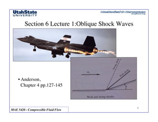
1. MAE 5420 - Compressible Fluid Flow!
1!
Section 6 Lecture 1:Oblique Shock Waves!
• Anderson, !
Chapter 4 pp.127-145 !

2. MAE 5420 - Compressible Fluid Flow!
2!
Mach Waves, Revisited!
• In Supersonic flow, pressure disturbances cannot !
outrun “point-mass” generating object!
• Result is an infinitesimally weak “mach wave”!
V t
c t
µ
sinµ =
c × t
V × t
"
#$
%
&' =
1
M
→ µ = sin−1 1
M

3. MAE 5420 - Compressible Fluid Flow!
3!
Oblique Shock Wave!
• When generating object is larger than a “point”, shockwave is stronger than!
mach wave …. Oblique shock wave!
• -- shock angle!
• -- turning or!
“wedge angle”!
β ≥ µ
β
θ
θ

4. MAE 5420 - Compressible Fluid Flow!
4!
Oblique Shock Wave Geometry!
! !Tangential ! !Normal!
Ahead ! !w1, Mt1 ! ! !u1, Mn1!
Of Shock!
Behind ! ! w2, Mt2 ! ! !u2, Mn2!
Shock !
• Must satisfy!
!i) continuity!
!ii) momentum!
!iii) energy!

5. MAE 5420 - Compressible Fluid Flow!
5!
Continuity Equation!
• For Steady Flow!
w2
u2
w1
u1
ds
ds
ρV
−>
• ds
−>
#
$
%
&
C.S.
∫∫ = 0 = −ρ1u1A + ρ2u2 A → ρ1u1 = ρ2u2
− ρV
−>
• ds
−>
#
$
%
&
C.S.
∫∫ =
∂
∂t
ρdv
c.v.
∫∫∫
#
$
)
%
&
*
0!

6. MAE 5420 - Compressible Fluid Flow!
6!
Momentum Equation!
• For Steady Flow w/no Body Forces!
ρV
−>
• ds
−>
#
$
%
&
C.S.
∫∫ V
−>
= − p( )
C.S.
∫∫ dS
−>
• Tangential Component!
• But from continuity!
−ρ1u1w1A + ρ2u2w2 A( )= 0
ρ1u1 = ρ2u2 w1 = w2
Tangential velocity is!
Constant across oblique!
Shock wave!

7. MAE 5420 - Compressible Fluid Flow!
7!
Momentum Equation (concluded)!
ρV
−>
• ds
−>
#
$
%
&
C.S.
∫∫ V
−>
= − p( )
C.S.
∫∫ dS
−>
• Normal Component! Tangential velocity is!
Constant across oblique!
Shock wave!
−ρ1u1
2
A + ρ2u2
2
A = p2 − p1( )A →
p1 + ρ1u1
2
= p2 + ρ2u2
2

8. MAE 5420 - Compressible Fluid Flow!
8!
Energy Equation!
• Steady Adiabatic Flow!
ρ e +
V2
2
"
#
$
%
&
' V
−>
• d S
−>
+ (pd S
−>
) • V
−>
C.S.
∫∫ = 0
C.S.
∫∫
• Tangential velocity components do not !
contribute to integrals … thus …!
p1u1 + ρ1 e1 +
V1
2
2
"
#
$
%
&
' u1 = p2u2 + ρ2 e2 +
V2
2
2
"
#
$
%
&
' u2

9. MAE 5420 - Compressible Fluid Flow!
9!
Energy Equation (cont’d)!
•!
• But …!
• … thus …!
Factor out {ρ1,u1}, {ρ2,u2}!
p1
ρ1
+ e1
"
#$
%
&' +
V1
2
2
(
)
*
*
+
,
-
-
ρ1u1 =
p2
ρ2
+ e2
"
#$
%
&' +
V2
2
2
(
)
*
*
+
,
-
-
ρ2u2
p1
ρ1
+ e1 = RgT1 + cvT1 = cp − cv( )T1 + cvT1 = cpT1 = h1
p2
ρ2
+ e2 = h2 … and …! ρ1u1 = ρ2u2
h1 +
V1
2
2
= h2 +
V2
2
2

10. MAE 5420 - Compressible Fluid Flow!
10!
Energy Equation (concluded)!
•!
• thus …!
Write Velocity in terms of components!
V1
2
= u1
2
+ w1
2
→ V2
2
= u2
2
+ w2
2
→ w1 = w2
h1 +
u1
2
2
= h2 +
u2
2
2

11. MAE 5420 - Compressible Fluid Flow!
11!
Collected Oblique Shock Equations!
• Continuity!
• Momentum!
• Energy!
w1 = w2
p1 + ρ1u1
2
= p2 + ρ2u2
2
ρ1u1 = ρ2u2
cpT1 +
u1
2
2
= cpT2 +
u2
2
2 θ
β−θ
β−θ
β
u1
u2
w1
w2

12. MAE 5420 - Compressible Fluid Flow!
12!
Compare Oblique to Normal Shock Equations!
• Continuity!
• Momentum!
• Energy!
ρ1V1 = ρ2V2
p1+ ρ1V1
2
= p2 + ρ2V2
2
cp1T1 +
V1
2
2
= cp2T2 +
V2
2
2
• Identical except for u1 replaces V1 (normal to shock wave)!
and w1=w2 (tangential to shock wave)!
Normal Shock Equations!

13. MAE 5420 - Compressible Fluid Flow!
13!
Compare Oblique to Normal Shock Equations"
(cont’d)!
• Defining:!
Mn
1=M1sin( )!
Mt
1=M1cos( )!
• Then by similarity!
we can write the solution!
Mn2 =
1+
γ −1( )
2
Mn1
2#
$%
&
'(
γ Mn1
2
−
γ −1( )
2
#
$%
&
'(
β
β

14. MAE 5420 - Compressible Fluid Flow!
14!
Compare Oblique to Normal Shock Equations"
(cont’d)!
• Similarity Solution!
ρ2
ρ1
=
γ +1( )Mn1
2
2 + γ −1( )Mn1
2
( )
p2
p1
= 1+
2γ
γ +1( )
Mn1
2
−1( )
T2
T1
= 1+
2γ
γ +1( )
Mn1
2
−1( )
#
$
%
&
'
(
2 + γ −1( )Mn1
2
( )
γ +1( )Mn1
2
#
$
%
%
&
'
(
(
Mn1 = M1 sin β( )
Letting!
Then …..!

15. MAE 5420 - Compressible Fluid Flow!
15!
Compare Oblique to Normal Shock Equations"
(cont’d)!
ρ2
ρ1
=
γ +1( ) M1 sinβ( )2
2 + γ −1( ) M1 sinβ( )2
( )
p2
p1
= 1+
2γ
γ +1( )
M1 sinβ( )2
−1( )
T2
T1
= 1+
2γ
γ +1( )
M1 sinβ( )2
−1( )%
&
'
(
)
*
2 + γ −1( ) M1 sinβ( )2
( )
γ +1( ) M1 sinβ( )2
%
&
'
'
(
)
*
*
Mn2 =
1+
γ −1( )
2
M1 sinβ( )2$
%&
'
()
γ M1 sinβ( )2
−
γ −1( )
2
$
%&
'
()
• Properties across Oblique Shock wave ~ f(M1, )!β

16. MAE 5420 - Compressible Fluid Flow!
16!
Total Mach Number Downstream "
of Oblique Shock!
w1 = w2
Tangential velocity is!
Constant across oblique!
Shock wave!
w1 = w2 → Mt1c1 = Mt2c2 = M1
cos(β)c1
Mt2 =
M1
cos(β)c1
c2
= M1
cos(β)
T1
T2
M2 = Mt2
2
+ Mn2
2
#$ %&

17. MAE 5420 - Compressible Fluid Flow!
17!
Total Mach Number Downstream "
of Oblique Shock (cont’d)!Tangential velocity is!
Constant across oblique!
Shock wave!
M2 = Mt2
2
+ Mn2
2
!" #$ → Mn2 =
1+
γ −1( )
2
M1
sin(β)[ ]2)
*+
,
-.
γ M1
sin(β)[ ]2
−
γ −1( )
2
)
*+
,
-.
M2 = M1
cos(β)[ ]2 T1
T2
+
1+
γ −1( )
2
M1
sin(β)[ ]2)
*+
,
-.
γ M1
sin(β)[ ]2
−
γ −1( )
2
)
*+
,
-.
!
"
/
/
/
/
#
$
0
0
0
0

18. MAE 5420 - Compressible Fluid Flow!
18!
Total Mach Number Downstream "
of Oblique Shock (concluded)!Tangential velocity is!
Constant across oblique!
Shock wave!
• Or … More simply .. If we consider geometric arguments!
M2 =
Mn2
sin β −θ( )
M3M2
Mn2
Mt2
β−θ

19. MAE 5420 - Compressible Fluid Flow!
19!
Oblique Shock Wave Angle!
• Properties across Oblique !
Shock wave ~ f(M1, )!
• is the geometric angle!
that “forces” the flow!
• How do we relate to ?!
β
θ β
θ

20. MAE 5420 - Compressible Fluid Flow!
20!
Oblique Shock Wave Angle (cont’d)!
• Since (from continuity)!
ρ1u1 = ρ2u2
θ
β−θ
β−θ
β
u1
u2
w1
w2
ρ1u1 = ρ2u2 →
u2
u1
=
ρ1
ρ2

21. MAE 5420 - Compressible Fluid Flow!
21!
Oblique Shock Wave Angle (cont’d)!
θ
β−θ
β−θ
β
u1
u2
w1
w2
u2
w2
= tan β −θ( )
u1
w1
= tan β( )
$
%
&
&
&
&
&
&
'
(
)
)
)
)
)
)
• from Momentum!
w1 = w2

22. MAE 5420 - Compressible Fluid Flow!
22!
Oblique Shock Wave Angle (cont’d)!
• Solving for the ratio u2/u1!
Implicit relationship for shock angle in terms of!
Free stream mach number and “wedge angle”!
→
u2
u1
=
tan β −θ( )
tan β( )
=
ρ1
ρ2
→→
ρ2
ρ1
=
γ +1( )Mn1
2
2 + γ −1( )Mn1
2
( )
∴
tan β −θ( )
tan β( )
=
2 + γ −1( ) M1 sin β( )() *+
2
( )
γ +1( ) M1 sin β( )() *+
2

23. MAE 5420 - Compressible Fluid Flow!
23!
Oblique Shock Wave Angle (cont’d)!
• Solve explicitly for tan( )!
tan β −θ( )
tan β( )
=
sin β −θ( )
cos β −θ( )
=
sin β( )cos θ( )− cos β( )sin θ( )
cos β( )cos θ( )+ sin β( )sin θ( )
$
%&
'
()
cosβ
sinβ
=
sin β( )cos θ( )
sinβ
−
cos β( )sin θ( )
sinβ
cos β( )cos θ( )
cosβ
+
sin β( )sin θ( )
cosβ
$
%
&
&
&
&
'
(
)
)
)
)
=
cos θ( )−
sin θ( )
tan β( )
cos θ( )+ tan β( )sin θ( )
$
%
&
&
&
&
'
(
)
)
)
)
=
1−
sin θ( )
cos θ( )tan β( )
1+
tan β( )sin θ( )
cos θ( )
$
%
&
&
&
&
'
(
)
)
)
)
=
1−
tan θ( )
tan β( )
1+ tan β( )tan θ( )
$
%
&
&
&
&
'
(
)
)
)
)
=
tan β( )− tan θ( )
tan β( )+ tan2
β( )tan θ( )
θ

24. MAE 5420 - Compressible Fluid Flow!
24!
Oblique Shock Wave Angle (cont’d)!
• Solve explicitly for tan( )!
tan β( )− tan θ( )
tan β( )+ tan2
β( )tan θ( )
=
2 + γ −1( ) M1 sin β( )%& '(
2
( )
γ +1( ) M1 sin β( )%& '(
2
θ

25. MAE 5420 - Compressible Fluid Flow!
25!
Oblique Shock Wave Angle (cont’d)!
• Solve for tan( )"
tan β( )− tan θ( )$% &' γ +1( ) M1 sin β( )$% &'
2
=
tan β( )+ tan2
β( )tan θ( )$% &' 2 + γ −1( ) M1 sin β( )$% &'
2
( )→
tan β( ) γ +1( ) M1 sin β( )$% &'
2
− 2 + γ −1( ) M1 sin β( )$% &'
2
( )$
%
&
'
=
tan θ( ) γ +1( ) M1 sin β( )$% &'
2
+ tan2
β( ) 2 + γ −1( ) M1 sin β( )$% &'
2
( )$
%
&
'
→
tan θ( ) =
tan β( ) γ +1( ) M1 sin β( )$% &'
2
− 2 + γ −1( ) M1 sin β( )$% &'
2
( )$
%
&
'
γ +1( ) M1 sin β( )$% &'
2
+ tan2
β( ) 2 + γ −1( ) M1 sin β( )$% &'
2
( )$
%
&
'
θ

26. MAE 5420 - Compressible Fluid Flow!
26!
Oblique Shock Wave Angle (cont’d)!
• Simplify Numerator"
tan β( ) γ +1( ) M1 sin β( )#$ %&
2
− 2 + γ −1( ) M1 sin β( )#$ %&
2
( )#
$
%
&
=
tan β( ) γ M1 sin β( )#$ %&
2
+ M1 sin β( )#$ %&
2
− 2 − γ M1 sin β( )#$ %&
2
+ M1 sin β( )#$ %&
2
#
$
%
&
=
tan β( ) 2 M1 sin β( )#$ %&
2
−1{ }#
$
%
&

27. MAE 5420 - Compressible Fluid Flow!
27!
Oblique Shock Wave Angle (cont’d)!
• Simplify Denominator"
γ +1( ) M1 sin β( )#$ %&
2
+ tan2
β( ) 2 + γ −1( ) M1 sin β( )#$ %&
2
( )#
$
%
&
=
tan2
β( ) γ +1( ) M1
sin β( )
tan β( )
#
$
(
%
&
)
2
+ 2 + γ −1( ) M1 sin β( )#$ %&
2
( )
#
$
(
(
%
&
)
)
=
tan2
β( ) γ +1( ) M1 cos β( )#$ %&
2
+ 2 + γ −1( ) M1 sin β( )#$ %&
2
( )#
$
%
&
=
tan2
β( ) γ +1( )M1
2
1− sin2
β( )#$ %& + 2 + γ −1( )M1
2
sin2
β( )#
$
%
& =
tan2
β( ) 2 + γ +1( )M1
2
− γ +1( )M1
2
sin2
β( )+ γ −1( )M1
2
sin2
β( )#$ %&#
$
%
& =
tan2
β( ) 2 + γ +1( )M1
2
− 2M1
2
sin2
β( )#$ %& = tan2
β( ) 2 + γ +1( )M1
2
− 2M1
2
sin2
β( )#$ %& =
tan2
β( ) 2 + γ M1
2
+ M1
2
1− 2sin2
β( )#$ %&#
$
%
& = tan2
β( ) 2 + γ M1
2
+ M1
2
cos2
β( )− sin2
β( )#$ %&#
$
%
& =
tan2
β( ) 2 + M1
2
γ + cos 2β( )#$ %&#$ %&

28. MAE 5420 - Compressible Fluid Flow!
28!
Oblique Shock Wave Angle (cont’d)!
• Collect terms"
tan θ( ) =
2tan β( ) M1 sin β( )#$ %&
2
−1{ }
tan2
β( ) 2 + M1
2
γ + cos 2β( )#$ %&#$ %&
=
2 M1
2
sin2
β( )−1{ }
tan β( ) 2 + M1
2
γ + cos 2β( )#$ %&#$ %&
• “Wedge Angle” Given explicitly as !
function of shock angle and freestream !
Mach number!
• Two Solutions “weak” and “strong” !
shock wave … in reality weak shock !
typically occurs; strong only occurs !
under very Specialized circumstances!
.e.g near stagnation point for a detached !
Shock (Anderson, pp. 138-139, 165,166) !

29. MAE 5420 - Compressible Fluid Flow!
29!
Oblique Shock Wave Angle (concluded)!
• Plotting versus "
M1=1.5! M1=2.0!
M1=2.5!
M1=3.0!
M1=5.0!
M1=4.0!
max!
curve!
“strong shock”!
“weak shock”!
β θ
γ = 1.4
θ

30. MAE 5420 - Compressible Fluid Flow!
15!
Compare Oblique to Normal Shock Equations"
(cont’d)!
ρ2
ρ1
=
γ +1( ) M1 sinβ( )2
2 + γ −1( ) M1 sinβ( )2
( )
p2
p1
= 1+
2γ
γ +1( )
M1 sinβ( )2
−1( )
T2
T1
= 1+
2γ
γ +1( )
M1 sinβ( )2
−1( )%
&
'
(
)
*
2 + γ −1( ) M1 sinβ( )2
( )
γ +1( ) M1 sinβ( )2
%
&
'
'
(
)
*
*
Mn2 =
1+
γ −1( )
2
M1 sinβ( )2$
%&
'
()
γ M1 sinβ( )2
−
γ −1( )
2
$
%&
'
()
• Properties across Oblique Shock wave ~ f(M1, )!β

31. MAE 5420 - Compressible Fluid Flow!
30!
Solving for Oblique Shock "
Wave Angle in Terms of Wedge Angle!
• As derived"
• “Wedge Angle” Given explicitly as function of shock !
angle and freestream Mach number!
• For most practical applications, the geometric deflection angle (wedge angle) and !
Mach number are prescribed .. Need in terms of and M1!
• Obvious Approach …. Numerical Solution using Newton’s method!
tan θ( ) =
2 M1
2
sin2
β( )−1{ }
tan β( ) 2 + M1
2
γ + cos 2β( )%& '(%& '(
β θ

32. MAE 5420 - Compressible Fluid Flow!
31!
Solving for Oblique Shock "
Wave Angle in Terms of Wedge Angle (cont’d)!
• Newton method"
2 M1
2
sin2
β( )−1{ }
tan β( ) 2 + M1
2
γ + cos 2β( )$% &'$% &'
− tan θ( ) ≡ f (β) = 0
f (β) = f (β( j) ) +
∂f
∂β
+
,-
.
/0
( j)
β − β( j)( )+ O(β2
) + ....→
β( j+1) = β( j) −
2 M1
2
sin2
β( )−1{ }
tan β( ) 2 + M1
2
γ + cos 2β( )$% &'$% &'
− tan θ( )
∂f
∂β
+
,-
.
/0
( j)

33. MAE 5420 - Compressible Fluid Flow!
32!
Solving for Oblique Shock "
Wave Angle in Terms of Wedge Angle (cont’d)!
• Newton method (continued)"
• Iterate until convergence!
∂f
∂β
=
2 M1
4
sin2
β( ) 1+ γ cos 2β( )$% &' + M1
2
2cos 2β( )+ γ −1( )+ 2$% &'
sin2
β( ) 2 + M1
2
γ + cos 2β( )$% &'$% &'
2

34. MAE 5420 - Compressible Fluid Flow!
33!
Solving for Oblique Shock "
Wave Angle in Terms of Wedge Angle (cont’d)!
∂f
∂β
β
• “Flat spot”!
Causes potential!
Convergence !
Problems with!
Newton Method!
Increasing!
Mach!

35. MAE 5420 - Compressible Fluid Flow!
34!
Solving for Oblique Shock "
Wave Angle in Terms of Wedge Angle (cont’d)!
• Newton method … Convergence can often be slow (because of low derivative slope)"
• Converged solution!
βtrue = 60.26o

36. MAE 5420 - Compressible Fluid Flow!
35!
Solving for Oblique Shock "
Wave Angle in Terms of Wedge Angle (concluded)!
• Newton method … or can “toggle” to strong shock solution"
• Strong !
shock solution!
βstrong = 71.87o

37. MAE 5420 - Compressible Fluid Flow!
36!
Solving for Oblique Shock "
Wave Angle in Terms of Wedge Angle (improved solution)!
• Because of the slow convergence of Newton’s method for this!
implicit function… explicit solution … !
(if possible) .. Or better behaved .. Method very desirable!
tan θ( ) =
2 M1
2
sin2
β( )−1{ }
tan β( ) 2 + M1
2
γ + cos 2β( )%& '(%& '(
=
2 M1
2
sin2
β( )−1{ }
tan β( ) 2 + γ M1
2
+ M1
2
cos2
β( )− sin2
β( )%& '(%
&
'
(
cos 2β( ) = cos2
β( )− sin2
β( )Substitute!

38. MAE 5420 - Compressible Fluid Flow!
37!
Solving for Oblique Shock "
Wave Angle in Terms of Wedge Angle (improved solution)"
(cont’d)!
• But, since! 1 = cos2
β( )+ sin2
β( )
2 M1
2
sin2
β( )−1{ }
tan β( ) 2 + γ M1
2
+ M1
2
cos2
β( )− sin2
β( )$% &'$
%
&
'
=
2 M1
2
sin2
β( )− sin2
β( )− cos2
β( ){ }
tan β( ) 2 + γ M1
2
+ M1
2
cos2
β( )− sin2
β( )$% &'$
%
&
'

39. MAE 5420 - Compressible Fluid Flow!
38!
Solving for Oblique Shock "
Wave Angle in Terms of Wedge Angle (improved solution)"
(cont’d)!
• Simplify and collect terms!
2 M1
2
sin2
β( )− sin2
β( )− cos2
β( ){ }
tan β( ) 2 + γ M1
2
+ M1
2
cos2
β( )− sin2
β( )$% &'$
%
&
'
=
M1
2
−1( )sin2
β( )− cos2
β( ){ }
tan β( ) 1+
γ
2
M1
2
+
1
2
M1
2
cos2
β( )− sin2
β( )$% &'
$
%(
&
')
=
M1
2
−1( )sin2
β( )− cos2
β( ){ }
tan β( ) 1+
γ
2
M1
2
+
1
2
M1
2
cos2
β( )− sin2
β( )$% &'
$
%(
&
')
=
M1
2
−1( )sin2
β( )− cos2
β( ){ }
tan β( ) 1+
γ + cos2
β( )− sin2
β( )
2
M1
2$
%
(
&
'
)

40. MAE 5420 - Compressible Fluid Flow!
39!
Solving for Oblique Shock "
Wave Angle in Terms of Wedge Angle (improved solution)"
(cont’d)!
• Again, Since!
M1
2
−1( )sin2
β( )− cos2
β( ){ }
tan β( ) 1+
γ + cos2
β( )− sin2
β( )
2
M1
2$
%
&
'
(
)
=
M1
2
−1( )sin2
β( )− cos2
β( ){ }
tan β( ) cos2
β( )+ sin2
β( )+
γ cos2
β( )+ sin2
β( )$% '( + cos2
β( )− sin2
β( )
2
M1
2
$
%
&
&
'
(
)
)
1 = cos2
β( )+ sin2
β( )

41. MAE 5420 - Compressible Fluid Flow!
40!
Solving for Oblique Shock "
Wave Angle in Terms of Wedge Angle (improved solution)"
(cont’d)!
• Regroup and collect terms!
M1
2
−1( )sin2
β( )− cos2
β( ){ }
tan β( ) cos2
β( )+ sin2
β( )+
γ cos2
β( )+ sin2
β( )$% &' + cos2
β( )− sin2
β( )
2
M1
2
$
%
(
(
&
'
)
)
=
M1
2
−1( )tan2
β( )−1{ }
tan β( ) 1+ tan2
β( )+
γ 1+ tan2
β( )$% &' +1− tan2
β( )
2
M1
2
$
%
(
(
&
'
)
)
=
M1
2
−1( )tan2
β( )−1{ }
tan β( ) 1+
γ +1
2
M1
2
+ tan2
β( )+
γ tan2
β( )$% &' − tan2
β( )
2
M1
2
$
%
(
(
&
'
)
)
=
M1
2
−1( )tan2
β( )−1{ }
tan β( ) 1+
γ +1
2
M1
2$
%(
&
') + tan2
β( ) 1+
γ −1
2
M1
2$
%(
&
')
$
%
(
&
'
)

42. MAE 5420 - Compressible Fluid Flow!
41!
Solving for Oblique Shock "
Wave Angle in Terms of Wedge Angle (improved solution)"
(cont’d)!
• Finally!
• Regrouping in terms of powers of tan( )!
tan θ( ) =
M1
2
−1( )tan2
β( )−1{ }
1+
γ +1
2
M1
2%
&'
(
)*tan β( )+ 1+
γ −1
2
M1
2%
&'
(
)*tan3
β( )
β
1+
γ −1
2
M1
2#
$%
&
'(tan θ( )
*
+
,
-
.
/
tan3
β( )− M1
2
−1( )tan2
β( )+ 1+
γ +1
2
M1
2#
$%
&
'(tan θ( )
*
+
,
-
.
/
tan β( )+1 = 0

43. MAE 5420 - Compressible Fluid Flow!
42!
Solving for Oblique Shock "
Wave Angle in Terms of Wedge Angle (improved solution)"
(cont’d)!
• Letting"
• Result is a cubic equation of the form!
a = 1+
γ −1
2
M1
2#
$%
&
'(tan θ( )
*
+
,
-
.
/
b = M1
2
−1( )
c = 1+
γ +1
2
M1
2#
$%
&
'(tan θ( )
*
+
,
-
.
/
x = tan β( )
ax3
− bx2
+ cx +1 = 0
• Polynomial has 3 real roots!
!i) weak shock!
!ii) strong shock!
!iii) meaningless solution!
! !( < 0)!β

44. MAE 5420 - Compressible Fluid Flow!
43!
Solving for Oblique Shock "
Wave Angle in Terms of Wedge Angle (improved solution)"
(cont’d)!
• Numerical Solution of Cubic (Newton’s method)!
ax3
− bx2
+ cx +1 ≡ f (x) = 0 →
0 = f (xj ) +
∂f (x)
∂x j
xj+1 − xj( )+ o(x2
)
xj+1 = xj −
f (xj )
∂f (x)
∂x j
= xj −
axj
3
− bxj
2
+ cxj +1
3axj
2
− 2bxj + c

45. MAE 5420 - Compressible Fluid Flow!
44!
Solving for Oblique Shock "
Wave Angle in Terms of Wedge Angle (improved solution)"
(cont’d)!
• Collecting terms!
xj −
axj
3
− bxj
2
+ cxj +1
3axj
2
− 2bxj + c
=
3axj
3
− 2bxj
2
+ cxj − axj
3
− bxj
2
+ cxj +1( )
3axj
2
− 2bxj + c
=
2axj
3
− bxj
2
−1
3axj
2
− 2bxj + c

46. MAE 5420 - Compressible Fluid Flow!
45!
Solving for Oblique Shock "
Wave Angle in Terms of Wedge Angle (improved solution)"
(cont’d)!
• Solution Algorithm (iterate to convergence)!
xj+1 =
2axj
3
− bxj
2
−1
3axj
2
− 2bxj + c
• Where again! a = 1+
γ −1
2
M1
2#
$%
&
'(tan θ( )
*
+
,
-
.
/
b = M1
2
−1( )
c = 1+
γ +1
2
M1
2#
$%
&
'(tan θ( )
*
+
,
-
.
/
x = tan β( )

47. MAE 5420 - Compressible Fluid Flow!
46!
Solving for Oblique Shock "
Wave Angle in Terms of Wedge Angle (improved solution)"
(cont’d)!
• Properties of Solver algorithm are much improved!
Improved Algorithm!Original Algorithm!
βtrue = 60.26o
• Original algorithm!
• Improved algorithm!

48. MAE 5420 - Compressible Fluid Flow!
47!
Solving for Oblique Shock "
Wave Angle in Terms of Wedge Angle (improved solution)"
(cont’d)!
• Three Solutions always returned depending on start condition!
Original Algorithm! Improved Algorithm!
βtrue = 60.26o
• Weak Shock Solution!

49. MAE 5420 - Compressible Fluid Flow!
48!
Solving for Oblique Shock "
Wave Angle in Terms of Wedge Angle (improved solution)"
(cont’d)!
• Three Solutions always returned depending on start condition!
Improved Algorithm!
• Strong Shock Solution!
βstrong = 71.87o

50. MAE 5420 - Compressible Fluid Flow!
49!
Solving for Oblique Shock "
Wave Angle in Terms of Wedge Angle (improved solution)"
(cont’d)!
• Three Solutions always returned depending on start condition!
Improved Algorithm!• Meaningless Solution! βmeaningless < 0o

51. MAE 5420 - Compressible Fluid Flow!
50!
Solving for Oblique Shock "
Wave Angle in Terms of Wedge Angle (explicit solution)"
Improved Algorithm!• Meaningless Solution!
• Explicit Solution … Using guidance from numerical algorithm, can we find!
Explicit (non -iterative) solution for shock angle?!
• Cubic equation has three explicit solutions!
!i) !weak shock!
!ii) !Strong shock!
!iii) !non-physical solution !

52. MAE 5420 - Compressible Fluid Flow!
51!
Solving for Oblique Shock "
Wave Angle in Terms of Wedge Angle (explicit solution)"
Improved Algorithm!
• Explicit Solution … Using guidance from numerical algorithm, can we find!
Explicit (non -iterative) solution for shock angle?!
• Root 1: tan[ ]=!
• Root 2: tan[ ]=!
• Root 3: tan[ ]=!
• Break solutions down into manageable form!
β
β
β

53. MAE 5420 - Compressible Fluid Flow!
52!
Solving for Oblique Shock "
Wave Angle in Terms of Wedge Angle (explicit solution)"
Improved Algorithm!• Meaningless Solution!
• Explicit Solution (From Anderson, pp. 142,143) …!
1+
γ −1
2
M1
2#
$%
&
'(tan θ( )
*
+
,
-
.
/
tan3
β( )− M1
2
−1( )tan2
β( )+ 1+
γ +1
2
M1
2#
$%
&
'(tan θ( )
*
+
,
-
.
/
tan β( )+1 = 0
tan β( ) =
M1
2
−1( )+ 2λ cos
4πδ + cos−1
χ( )
3
'
()
*
+,
3 1+
γ −1
2
M1
2.
/0
1
23tan θ( )
λ = M1
2
−1( )
2
− 3 1+
γ −1
2
M1
2$
%&
'
() 1+
γ +1
2
M1
2$
%&
'
()tan2
θ( )
χ =
M1
2
−1( )
3
− 9 1+
γ −1
2
M1
2$
%&
'
() 1+
γ −1
2
M1
2
+
γ +1
4
M1
4$
%&
'
()tan2
θ( )
λ3
δ = 0 ---> Strong Shock!
δ = 1 ---> Weak Shock !

54. MAE 5420 - Compressible Fluid Flow!
53!
Solving for Oblique Shock "
Wave Angle in Terms of Wedge Angle (explicit solution)"
Improved Algorithm!• Meaningless Solution!
• Explicit Solution Check … let {M=5, , =40°}!
λ = M1
2
−1( )
2
− 3 1+
γ −1
2
M1
2$
%&
'
() 1+
γ +1
2
M1
2$
%&
'
()tan2
θ( ) =!
= 13.5321!
5
2
1−( )
2
3 1
1.4 1−
2
5
2
+" #
$ % 1
1.4 1+
2
5
2
+" #
$ % π
180
40" #
$ %tan" #
$ %
2
−
" #
' (
$ % 0.5
θγ = 1.4

55. MAE 5420 - Compressible Fluid Flow!
54!
Solving for Oblique Shock "
Wave Angle in Terms of Wedge Angle (explicit solution)"
Improved Algorithm!• Meaningless Solution!
• Explicit Solution Check … let {M=5, , =40°}!
=!
χ =
M1
2
−1( )
3
− 9 1+
γ −1
2
M1
2$
%&
'
() 1+
γ −1
2
M1
2
+
γ +1
4
M1
4$
%&
'
()tan2
θ( )
λ3
= -0.267118!
52
1−( )
3
9 1
1.4 1−
2
52
+" #
$ % 1
1.4 1−
2
52 1.4 1+
4
54
+ +" #
$ % π
180
40" #
$ %tan" #
$ %
2
−
13.5321
3
θγ = 1.4

56. MAE 5420 - Compressible Fluid Flow!
55!
Solving for Oblique Shock "
Wave Angle in Terms of Wedge Angle (explicit solution)"
Improved Algorithm!• Meaningless Solution!
tan β( ) =
M1
2
−1( )+ 2λ cos
4πδ + cos−1
χ( )
3
'
()
*
+,
3 1+
γ −1
2
M1
2.
/0
1
23tan θ( )
δ = 1 ---> Weak Shock !
=!
180
π
5
2
1−( ) 2 13.5321( )
4π 1( ) 0.26712−( )acos+
3
# $
% &cos+
3 1
1.4 1−
2
5
2
+# $
% & π
180
40# $
% &tan
# $
' (
' (
' (
' (
% &
atan
= 60.259°! Check!!
• Explicit Solution Check … let {M=5, , =40°}!θγ = 1.4

57. MAE 5420 - Compressible Fluid Flow!
56!
Solving for Oblique Shock "
Wave Anglein Terms of Wedge Angle (explicit solution)"
• Meaningless Solution!
tan β( ) =
M1
2
−1( )+ 2λ cos
4πδ + cos−1
χ( )
3
'
()
*
+,
3 1+
γ −1
2
M1
2.
/0
1
23tan θ( )
δ = 0 ---> Strong Shock !
=!
= 71.869°! Check!!
180
π
5
2
1−( ) 2 13.5321( )
4π 0( ) 0.26712−( )acos+
3
# $
% &cos+
3 1
1.4 1−
2
5
2
+# $
% & π
180
40# $
% &tan
# $
' (
' (
' (
' (
% &
atan
… OK .. This works …. But is it !
… the best method?!
(concluded)!
• Explicit Solution Check … let {M=5, , =40°}!θγ = 1.4

58. MAE 5420 - Compressible Fluid Flow!
57!
Floating Point Operation (FLOP) Estimate!
tan β( ) =
M1
2
−1( )+ 2λ cos
4πδ + cos−1
χ( )
3
'
()
*
+,
3 1+
γ −1
2
M1
2.
/0
1
23tan θ( )
tan θ( )=
M1
2
−1( )tan2
β( )−1{ }
1+
γ +1
2
M1
2%
&'
(
)*tan β( )+ 1+
γ −1
2
M1
2%
&'
(
)*tan3
β( )
xj+1 =
2axj
3
− bxj
2
−1
3axj
2
− 2bxj + c
• Actually the simplified numerical!
Algorithm is slightly faster than closed!
Form solution !

59. MAE 5420 - Compressible Fluid Flow!
58!
Oblique Shock Waves:"
Collected Algorithm!
• Properties across Oblique !
Shock wave ~ f(M1, )!
• is the geometric angle!
that “forces” the flow!
tan θ( ) =
2 M1
2
sin2
β( )−1{ }
tan β( ) 2 + M1
2
γ + cos 2β( )%& '(%& '(
θ
β

60. MAE 5420 - Compressible Fluid Flow!
59!
Oblique Shock Waves:"
Collected Algorithm (cont’d)!
• Can be re-written as third order polynomial in tan( )!
• “Very Easy” numerical solution!
xj+1 =
2axj
3
− bxj
2
−1
3axj
2
− 2bxj + c
a = 1+
γ −1
2
M1
2#
$%
&
'(tan θ( )
*
+
,
-
.
/
b = M1
2
−1( )
c = 1+
γ +1
2
M1
2#
$%
&
'(tan θ( )
*
+
,
-
.
/
x = tan β( )
• Cubic equation has three solutions!
!i) !weak shock!
!ii) !Strong shock!
!iii) !non-physical solution !
θ
1+
γ −1
2
M1
2#
$%
&
'(tan θ( )
*
+
,
-
.
/
tan3
β( )− M1
2
−1( )tan2
β( )+ 1+
γ +1
2
M1
2#
$%
&
'(tan θ( )
*
+
,
-
.
/
tan β( )+1 = 0

61. MAE 5420 - Compressible Fluid Flow!
60!
Oblique Shock Waves:"
Collected Algorithm (cont’d)!
• “Less Obvious” explicit solution!
tan β( ) =
M1
2
−1( )+ 2λ cos
4πδ + cos−1
χ( )
3
'
()
*
+,
3 1+
γ −1
2
M1
2.
/0
1
23tan θ( )
λ = M1
2
−1( )
2
− 3 1+
γ −1
2
M1
2$
%&
'
() 1+
γ +1
2
M1
2$
%&
'
()tan2
θ( )
χ =
M1
2
−1( )
3
− 9 1+
γ −1
2
M1
2$
%&
'
() 1+
γ −1
2
M1
2
+
γ +1
4
M1
4$
%&
'
()tan2
θ( )
λ3
δ = 0 ---> Strong Shock!
δ = 1 ---> Weak Shock !
• Either solution!
Method is acceptable!
For large scale-calculations!

62. MAE 5420 - Compressible Fluid Flow!
61!
Oblique Shock Waves:"
Collected Algorithm (cont’d)!
• ... and the rest of the story … !
ρ2
ρ1
=
γ +1( ) M1 sinβ( )2
2 + γ −1( ) M1 sinβ( )2
( )
p2
p1
= 1+
2γ
γ +1( )
M1 sinβ( )2
−1( )
T2
T1
= 1+
2γ
γ +1( )
M1 sinβ( )2
−1( )%
&
'
(
)
*
2 + γ −1( ) M1 sinβ( )2
( )
γ +1( ) M1 sinβ( )2
%
&
'
'
(
)
*
*

63. MAE 5420 - Compressible Fluid Flow!
62!
Oblique Shock Waves:"
Collected Algorithm (concluded)!
• ... and the rest of the story … !
Mn2 =
1+
γ −1( )
2
M1 sinβ( )2$
%&
'
()
γ M1 sinβ( )2
−
γ −1( )
2
$
%&
'
()
M2 =
Mn2
sin β −θ( )
P02
P01
=
2
γ +1( ) γ M1 sinβ( )2
−
γ −1( )
2
$
%&
'
()
1
γ −1
γ +1( )
2
M1 sinβ( )
*
+
,
-
.
/
2
1+
γ −1
2
M1 sinβ( )2$
%&
'
()
$
%
&
&
&
&
'
(
)
)
)
)
γ
γ −1
$
%&
'
()

64. MAE 5420 - Compressible Fluid Flow!
63!
Example:!
•M1 = 3.0, p1=1atm, T1=288°K, =20°, =1.4, !
β
θ
M1
M2
• Compute shock wave angle (weak)!
• Compute P02, T02, p2, T2, M2 … Behind Shockwave!
θ γ

65. MAE 5420 - Compressible Fluid Flow!
64!
Example: (cont’d)!
•M1 = 3.0, p1=1atm, =1.4, T1=288°K,
=20°!
• Explicit Solver for !
λ = M1
2
−1( )
2
− 3 1+
γ −1
2
M1
2$
%&
'
() 1+
γ +1
2
M1
2$
%&
'
()tan2
θ( ) =7.13226!
χ =
M1
2
−1( )
3
− 9 1+
γ −1
2
M1
2$
%&
'
() 1+
γ −1
2
M1
2
+
γ +1
4
M1
4$
%&
'
()tan2
θ( )
λ3
=0.93825!
θ
γ
β

66. MAE 5420 - Compressible Fluid Flow!
65!
Example: (cont’d)!
•M1 = 3.0, p1=1atm, =1.4, T1=288°K, =20°!
• = 1 (weak shock)!
180
π
3
2
1− 2 7.13226
4π 1( ) 0.93825( )acos+
3
# $
% &cos⋅+
3 1
1.4 1−
2
3
2
+# $
% & π
180
20# $
% &tan
# $
( )
( )
( )
( )
% &
atan
tan β( ) =
M1
2
−1( )+ 2λ cos
4πδ + cos−1
χ( )
3
'
()
*
+,
3 1+
γ −1
2
M1
2.
/0
1
23tan θ( )
=!
37.764°!
θγ
δ

67. MAE 5420 - Compressible Fluid Flow!
66!
Example: (cont’d)!
•M1 = 3.0, p1=1atm, =1.4, T1=288°K, =20°!
• Compute Normal Component of Free stream mach Number!
Mn1 = M1 sinβ = 3
π
180
37.7636" #
$ %sin =1.837!
Normal Shock Solver!
• Mach “normal” component of number behind shock wave!
θγ
Mn2
2
#$ → Mn2 =
1+
γ −1( )
2
M1
sin(β)[ ]2)
*+
,
-.
γ M1
sin(β)[ ]2
−
γ −1( )
2
)
*+
,
-.
2 T1
1+
γ −1( )
2
M1
sin(β)[ ]2)
*+
,
-.
#
0
0
=0.608392!

68. MAE 5420 - Compressible Fluid Flow!
67!
Example: (cont’d)!
•M1 = 3.0, p1=1atm, =1.4, T1=288°K, =20°!
• Mach “normal” component of number behind shock wave!
θγ
Mn2
2
#$ → Mn2 =
1+
γ −1( )
2
M1
sin(β)[ ]2)
*+
,
-.
γ M1
sin(β)[ ]2
−
γ −1( )
2
)
*+
,
-.
s(β)]2 T1
T2
+
1+
γ −1( )
2
M1
sin(β)[ ]2)
*+
,
-.
γ M1
sin(β)[ ]2
−
γ −1( )
2
)
*+
,
-.
#
$
0
0
0
0
=0.608392!
M2 =
Mn2
sin β −θ( ) M3M2
Mn2
Mt2
β−θ
=1.99414!
FLOW BEHIND SHOCK WAVE IS SUPERSONIC!!

69. MAE 5420 - Compressible Fluid Flow!
68!
Example: (cont’d)!
•M1 = 3.0, p1=1atm, =1.4, T1=288°K, =20°!
• Compute Normal Component of Free stream mach Number!
p2
p1
= 1+
2γ
γ +1( )
Mn1
2
−1( )
Mn1 = M1 sinβ = 3
π
180
37.7636" #
$ %sin =1.837!
Normal Shock Solver!
p2 = 3.771(1 atm) = 3.771 atm !
• Compute Pressure ratio across shock!
• Flow is compressed!
θγ

70. MAE 5420 - Compressible Fluid Flow!
69!
Example: (cont’d)!
•M1 = 3.0, p1=1atm, =1.4, T1=288°K, =20°!
• Compute Temperature ratio Across Shock!
Normal Shock Solver!
T2 = 1.5596(288 °K) = 449.2 °K !
T2
T1
= 1+
2γ
γ +1( )
Mn1
2
−1( )
#
$
%
&
'
(
2 + γ −1( )Mn1
2
( )
γ +1( )Mn1
2
#
$
%
%
&
'
(
(
θγ

71. MAE 5420 - Compressible Fluid Flow!
70!
Example: (cont’d)!
•M1 = 3.0, p1=1atm, =1.4, T1=288°K, =20°!
• Compute Stagnation Pressure ratio across shock!
Normal Shock Solver!
0.7961!
Mn1 = M1 sinβ = 3
π
180
37.7636" #
$ %sin =1.837!
P02
P01
=
θγ

72. MAE 5420 - Compressible Fluid Flow!
71!
Example: (cont’d)!
•M1 = 3.0, p1=1atm, =1.4, T1=288°K, =20°!
• Compute Stagnation Pressure ratio (alternate method)!
2
1.4 1+( ) 1.4 3
π
180
37.7636" #
$ %sin" #
$ %
2
1.4 1−( )
2" #
$ %−
" #
' (
$ %
1
1.4 1−
1.4 1+( )
2
" #
$ %
2
3
π
180
37.7636" #
$ %sin" #
$ %
2
" #
' (
$ %
1
1.4 1−( )
2
" #
$ % 3
π
180
37.7636" #
$ %sin" #
$ %
2
+
" #
' (
$ %
" #
' (
' (
' (
' (
$ %
1.4
1.4 1−( )
=0.7961!
θγ
P02
P01
=
2
γ +1( ) γ Mn1
2
−
γ −1( )
2
#
$%
&
'(
1
γ −1
γ +1( )
2
Mn1
)
*
+
,
-
.
2
1+
γ −1
2
Mn1
2#
$%
&
'(
#
$
%
%
%
%
&
'
(
(
(
(
γ
γ −1
#
$%
&
'(

73. MAE 5420 - Compressible Fluid Flow!
72!
Example: (cont’d)!
•M1 = 3.0, p1=1atm, =1.4, T1=288°K, =20°!
• Compute Stagnation Pressure!
=29.24 atm!
P02
=
P02
P01
×
P01
p1
× p1
=
P02
P01
× 1+
γ −1
2
M1
2$
%&
'
()
γ
γ −1
× p1
0.7961( ) 1+
1.4 −1
2
32$
%&
'
()
1.4
1.4−1
×1atm =
θγ

74. MAE 5420 - Compressible Fluid Flow!
73!
Example: (cont’d)!
•M1 = 3.0, p1=1atm, =1.4, T1=288°K, =20°!
• Compute Stagnation Temperature behind shock!
=806.4 oK!
T02
= T01
=
T01
T1
× T1
= 1+
γ −1
2
M1
2$
%&
'
() × T1
1+
1.4 −1
2
32$
%&
'
() × 288o
K =
θγ

75. MAE 5420 - Compressible Fluid Flow!
74!
Example: (summary)!
Ahead of shock Behind Shock
M∞ = 3.0 M2 =1.99414
θ = 200
β = 37.764o
p∞ =1 atm p2 = 3.771 atm
T∞ = 288o
K T2 = 449.2o
K
P0∞
= 36.73 atm P02
= 29.24 atm
T0θ
= 806.4o
K T02
= 806.4o
K
M1n
=1.837 M2n
= 0.608392
M1t
= 2.372 M2t
=1.21333
Flow is supersonic!
Behind shock wave!

76. MAE 5420 - Compressible Fluid Flow!
75!
What Happens When …. !
Flow is subsonic!
Behind shock wave!
θ = 34.01o ?!
β = 63.786o
→ M1n
= 3⋅sin(
π
180
63.786o
) = 2.69145 → M2 n
= 0.49631
M2 =
M2 n
sin β −θ( )
=
0.49631
sin(
π
180
63.786o
− 34.01o
)
= 0.999394
Select Weak Shock Wave Solution!
Select Strong Shock Wave Solution!
β = 66.6448o
→ M1n
= 3⋅sin(
π
180
63.786o
) = 2.75419 → M2 n
= 0.491498
M2 =
M2 n
sin β −θ( )
=
0.491498
sin(
π
180
63.786o
− 34.01o
)
= 0.989705

77. MAE 5420 - Compressible Fluid Flow!
76!
Add another Curve to β-θ-M diagram…. !
M2 “sonic line”!

78. MAE 5420 - Compressible Fluid Flow!
Weak, Strong, and Detached Shockwaves!
77!

79. MAE 5420 - Compressible Fluid Flow!
78!
What Happens when … !
•M1 = 3.0, p1=1atm, =1.4, T1=288°K, =0.00001°!
• Explicit Solver for !
λ = M1
2
−1( )
2
− 3 1+
γ −1
2
M1
2$
%&
'
() 1+
γ +1
2
M1
2$
%&
'
()tan2
θ( ) =8.0!
χ =
M1
2
−1( )
3
− 9 1+
γ −1
2
M1
2$
%&
'
() 1+
γ −1
2
M1
2
+
γ +1
4
M1
4$
%&
'
()tan2
θ( )
λ3
=1.0!
θγ
β

80. MAE 5420 - Compressible Fluid Flow!
79!
What Happens when (cont’d) !
•M1 = 3.0, p1=1atm, =1.4, T1=288°K, =0.00001°!
tan β( ) =
M1
2
−1( )+ 2λ cos
4πδ + cos−1
χ( )
3
'
()
*
+,
3 1+
γ −1
2
M1
2.
/0
1
23tan θ( )
=19.47°! µ =
180
π
sin−1 1
M1
#
$
%
&
'
( = 19.47o
• “mach line”!
θγ
β

81. MAE 5420 - Compressible Fluid Flow!
80!
What Happens when (cont’d) !
•M1 = 3.0, p1=1atm, =1.4, T1=288°K, =0.00001°!
• Χοµπυτε Normal Component of Free stream mach Number!
Mn1 = M1 sinβ = 1.0000!
• !
p2
p1
= 1+
2γ
γ +1( )
Mn1
2
−1( ) = 1.0 (NO COMPRESSION!)!
θγ

82. MAE 5420 - Compressible Fluid Flow!
81!
Expansion Waves !
• So if!
! >0 .. Compression around corner!
! =0 … no compression across shock!
β
θ
M1
M2
θ
θ

83. MAE 5420 - Compressible Fluid Flow!
82!
Expansion Waves (concluded) !
• Then it follows that!
! <0 .. We get an expansion wave!
• Next!
!Prandtl-Meyer !
!Expansion waves!
θ