Unit 3.2

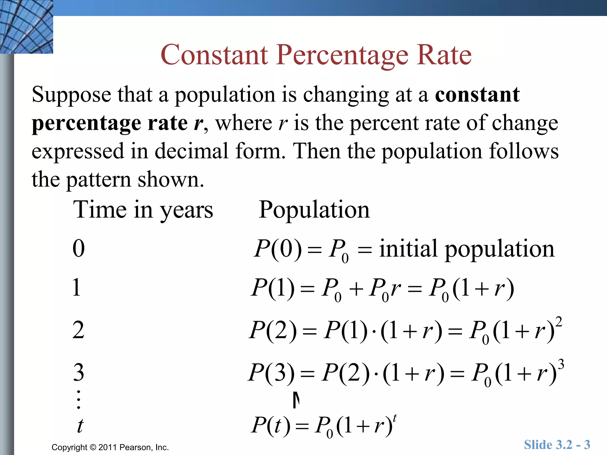
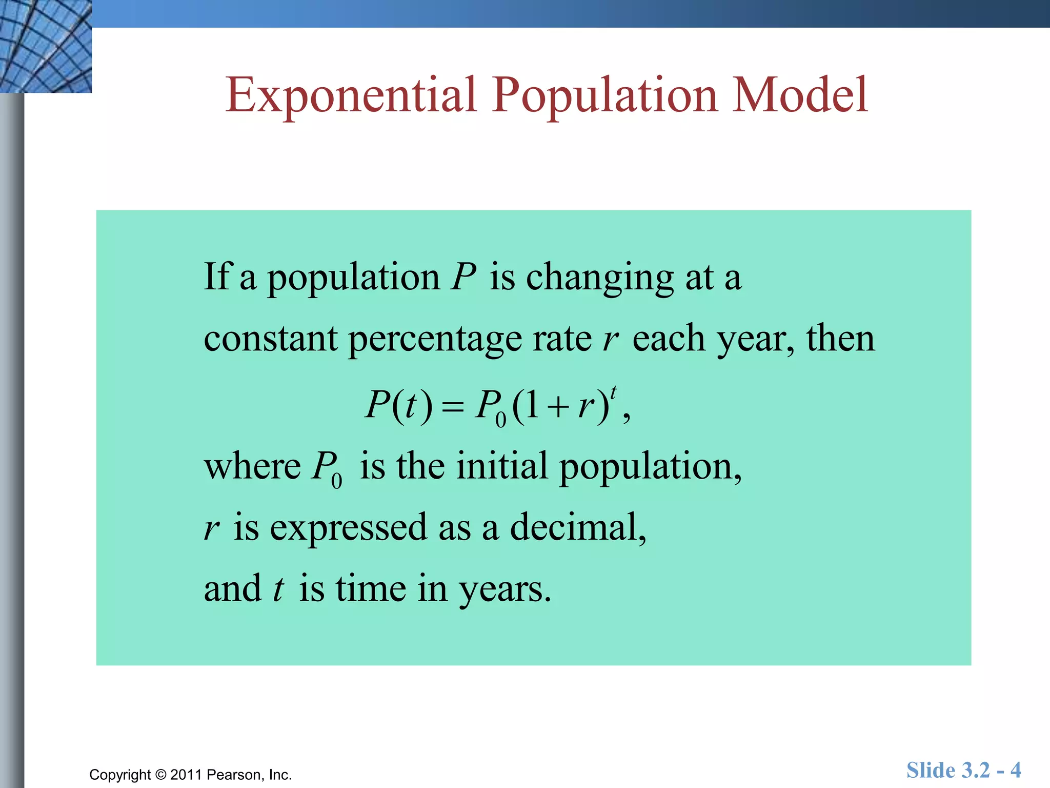
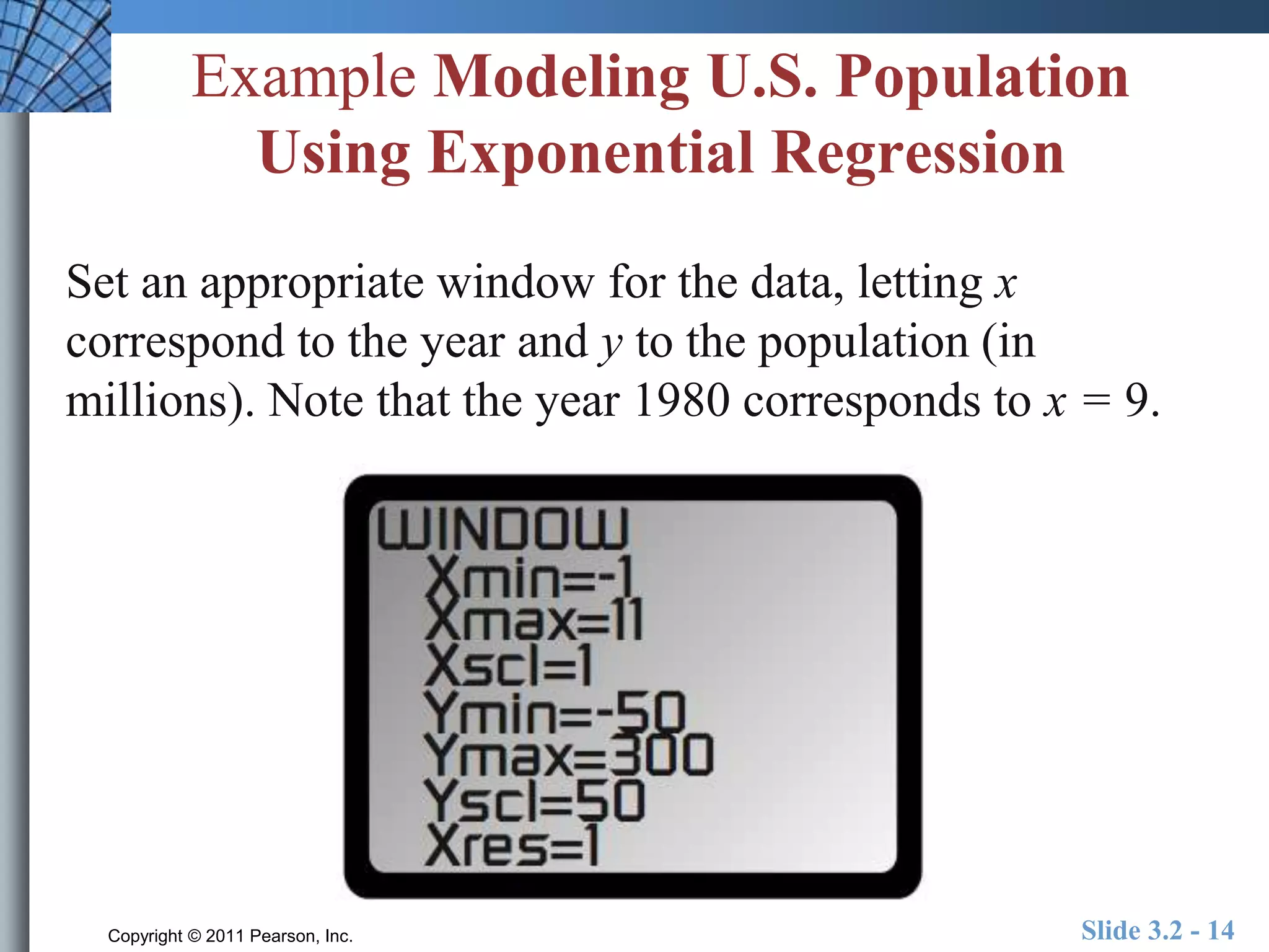
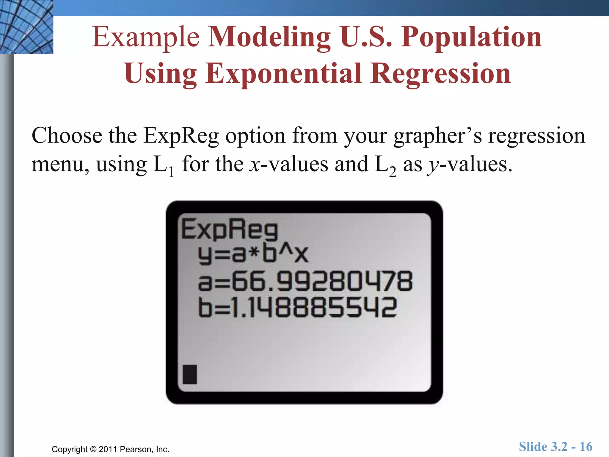
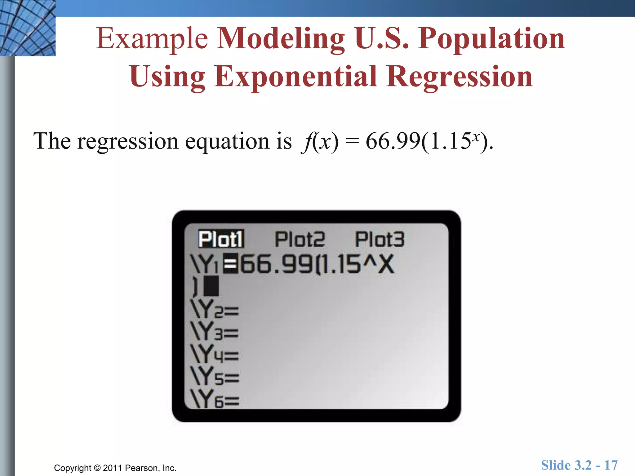
3.2
Exponential
and Logistic
Modeling
Copyright © 2011 Pearson, Inc.

What you’ll learn about
 Constant Percentage Rate and Exponential Functions
 Exponential Growth and Decay Models
 Using Regression to Model Population
 Other Logistic Models
… and why
Exponential functions model many types of unrestricted
growth; logistic functions model restricted growth,
including the spread of disease and the spread of rumors.
Copyright © 2011 Pearson, Inc. Slide 3.2 - 2

Constant Percentage Rate
Suppose that a population is changing at a constant
percentage rate r, where r is the percent rate of change
expressed in decimal form. Then the population follows
the pattern shown.
Time in years Population
0 P(0)  P0  initial population
1 P(1)  P0  P0r  P0 (1 r)
2 P(2)  P(1)  (1 r)  P0 (1 r)2
3 P(3)  P(2)  (1 r)  P0 (1 r)3
M
t P(t)  P0 (1 r)t

Exponential Population Model
If a population P is changing at a
constant percentage rate r each year, then
P(t )  P0 (1 r)t ,
where P0 is the initial population,
r is expressed as a decimal,
and t is time in years.

Example Finding Growth and Decay
Rates
Tell whether the population model P(t )  786,5431.021t
is an exponential growth function or exponential decay
function, and find the constant percent rate of growth.

Example Finding Growth and Decay
Rates
Tell whether the population model P(t )  786,5431.021t
is an exponential growth function or exponential decay
function, and find the constant percent rate of growth.
Because 1 r  1.021, r  .021  0.
So, P is an exponential growth function
with a growth rate of 2.1%.

Example Finding an Exponential
Function
Determine the exponential function with initial
value = 10, increasing at a rate of 5% per year.

Example Finding an Exponential
Function
Determine the exponential function with initial
value = 10, increasing at a rate of 5% per year.
Because P0  10 and r  5% 0.05, the function is
P(t )  10(1 0.05)t or P(t )  10(1.05)t .

Example Modeling Bacteria Growth
Suppose a culture of 200 bacteria is put into a petri dish
and the culture doubles every hour.
Predict when the number of bacteria will be 350,000.

Example Modeling Bacteria Growth
Suppose a culture of 200 bacteria is put into a petri dish
and the culture doubles every hour.
Predict when the number of bacteria will be 350,000.
represents the bacteria population t hr
after it is placed in the petri dish.
To find out when the population will
reach 350,000, solve 350,000  200  2t
for t using a calculator.
400  200  2
800  200  22
M
P(t )  200  2t
t  10.77 or about 10 hours and 46 minutes.

Example Modeling U.S. Population
Using Exponential Regression
Use the population data in
the table to predict the
population for the year
2000. Compare with the
actual 2000 population of
approximately 281
million.

Let x = 0 represent 1890,
x = 1 represent 1900, and
so on. The year 2000 is
represented by x = 11.
Create a scatter plot of the
data following the steps
below.

Enter the data into the statistical memory of your
grapher.

Set an appropriate window for the data, letting x
correspond to the year and y to the population (in
millions). Note that the year 1980 corresponds to x = 9.

Make a scatter plot.

Choose the ExpReg option from your grapher’s regression
menu, using L1 for the x-values and L2 as y-values.

The regression equation is f(x) = 66.99(1.15x).

Graph both the scatter plot and the regression equation.
Use the CALC-VALUE option to find f (11).

The year 2000 is represented by x =11, and
f (11) = 311.66.
Interpret This exponential model estimates
the 2000 population to be 311.66 million, an
overestimate of approximately 31 million.

Maximum Sustainable Population
Exponential growth is unrestricted, but
population growth often is not. For many
populations, the growth begins exponentially,
but eventually slows and approaches a limit to
growth called the maximum sustainable
population.

Example Modeling a Rumor
A high school has 1500 students. 5 students start a rumor,
which spreads logistically so that S(t )  1500 / (1 29  e-0.9t )
models the number of students who have heard the rumor
by the end of t days, where t  0 is the day the rumor
begins to spread.
(a) How many students have heard the rumor by the
end of Day 0?
(b) How long does it take for 1000 students to hear
the rumor?

5 students start a rumor, S(t )  1500 / (1 29  e-0.9t )
where t  0 is the day the rumor begins to spread.
(a) How many students have heard the rumor by the
end of Day 0?
(a) S(0)  1500 / (1 29  e-0.9(0) )
 1500 / (1 29 1)
 1500 / 30  50.
So 50 students have heard the rumor
by the end of day 0.

5 students start a rumor, S(t )  1500 / (1 29  e-0.9t )
where t  0 is the day the rumor begins to spread.
(b) How long does it take for 1000 students to hear
the rumor?
Solve 1000  1500 / (1 29  e-0.9t ) for t.
t  4.5. So 1000 students have heard the
rumor half way through the fifth day.

Quick Review
Convert the percent to decimal form or the decimal into
a percent.
1. 16%
2. 0.05
3. Show how to increase 25 by 8% using a single
multiplication.
Solve the equation algebraically.
4. 20 b2  720
Solve the equation numerically.
5. 123b3  7.872

Quick Review Solutions
Convert the percent to decimal form or the decimal into
a percent.
1. 16% 0.16
2. 0.05 5%
3. Show how to increase 25 by 8% using a single
multiplication.
Solve the equation algebraically. 25 1.08
4. 20 b2  720  6
Solve the equation numerically.
5. 123b3  7.872 0.4

Unit 3.2

More Related Content

What's hot

Similar to Unit 3.2

More from Mark Ryder

Recently uploaded

Unit 3.2