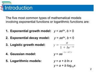
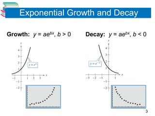
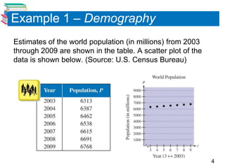
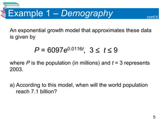
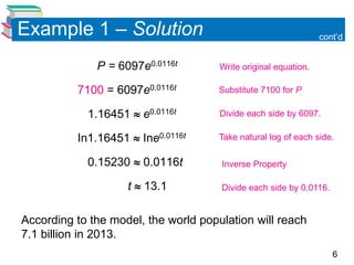
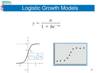
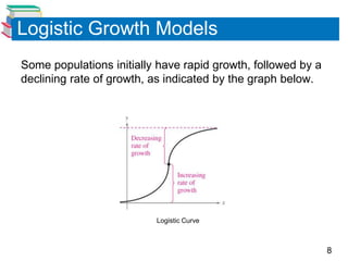
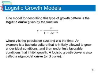
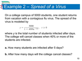
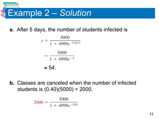
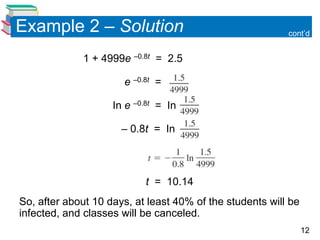
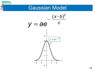
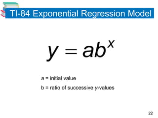
The document discusses various mathematical models involving exponential and logarithmic functions, including exponential growth and decay models, logistic growth models, Gaussian models, and logarithmic models. It provides examples of how each type of model can be used, such as modeling world population growth with an exponential function, modeling the spread of a virus on a college campus with a logistic function, and modeling cooling of a heated object using Newton's Law of Cooling. The document also discusses how to graph and solve problems involving these different mathematical models.

1. Exponential and
3.5 Logarithmic Models

2. Introduction
The five most common types of mathematical models
involving exponential functions or logarithmic functions are:
1. Exponential growth model: y = aebx, b > 0
2. Exponential decay model: y = aebx, b < 0
3. Logistic growth model:
4. Gaussian model: y = ae
5. Logarithmic models: y = a + b ln x
y = a + b log10x
2

3. Exponential Growth and Decay
Growth: y = aebx, b > 0 Decay: y = aebx, b < 0
3

4. Example 1 – Demography
Estimates of the world population (in millions) from 2003
through 2009 are shown in the table. A scatter plot of the
data is shown below. (Source: U.S. Census Bureau)
4

5. Example 1 – Demography cont’d
An exponential growth model that approximates these data
is given by
P = 6097e0.0116t, 3  t  9
where P is the population (in millions) and t = 3 represents
2003.
a) According to this model, when will the world population
reach 7.1 billion?
5

6. Example 1 – Solution cont’d
P = 6097e0.0116t Write original equation.
7100 = 6097e0.0116t Substitute 7100 for P.
1.16451  e0.0116t Divide each side by 6097.
In1.16451  Ine0.0116t Take natural log of each side.
0.15230  0.0116t Inverse Property
t  13.1 Divide each side by 0.0116.
According to the model, the world population will reach
7.1 billion in 2013.
6

7. Logistic Growth Models
7

8. Logistic Growth Models
Some populations initially have rapid growth, followed by a
declining rate of growth, as indicated by the graph below.
Logistic Curve
8

9. Logistic Growth Models
One model for describing this type of growth pattern is the
logistic curve given by the function
where y is the population size and x is the time. An
example is a bacteria culture that is initially allowed to grow
under ideal conditions, and then under less favorable
conditions that inhibit growth. A logistic growth curve is also
called a sigmoidal curve (or S curve).
9

10. Example 2 – Spread of a Virus
On a college campus of 5000 students, one student returns
from vacation with a contagious flu virus. The spread of the
virus is modeled by
where y is the total number of students infected after days.
The college will cancel classes when 40% or more of the
students are infected.
a. How many students are infected after 5 days?
b. After how many days will the college cancel classes?
10

11. Example 2 – Solution
a. After 5 days, the number of students infected is
 54.
b. Classes are canceled when the number of infected
students is (0.40)(5000) = 2000.
11

12. Example 2 – Solution cont’d
1 + 4999e –0.8t = 2.5
e –0.8t =
In e –0.8t = In
– 0.8t = In
t = 10.14
So, after about 10 days, at least 40% of the students will be
infected, and classes will be canceled.
12

13. Gaussian Model
( x b)
2

y ae c
13

14. Gaussian Models
This type of model is commonly used in probability and
statistics to represent populations that are normally
distributed. For standard normal distributions, the model
takes the form
The graph of a Gaussian model is called a bell-shaped
curve. Try graphing the normal distribution curve with a
graphing utility. Can you see why it is called a bell-
shaped curve?
14

15. Gaussian Models
The average value for a population can be found from the
bell-shaped curve by observing where the maximum
y-value of the function occurs. The x-value corresponding
to the maximum y-value of the function represents the
average value of the independent variable—in this case, x.
15

16. Example 3 – SAT Scores
In 2009, the Scholastic Aptitude Test (SAT) mathematics
scores for college-bound seniors roughly followed the
normal distribution
( x 515)2

y  0.0034e 26,912
, 200  x  800
where x is the SAT score for mathematics.
a) Use a graphing utility to graph this function
b) Estimate the average SAT score.
16

17. Example 3 – Solution
On this bell-shaped curve, the maximum value of the curve
represents the average score. Using the maximum feature of
the graphing utility, you can see that the average mathematics
score for college bound seniors in 2009 was 515.
17

18. Logarithmic Models
y = a + b ln x y = a + b log10x
18

19. Example 4 - Meteorology
In meteorology, the relationship between the height H of a
weather balloon (measured in km) and the atmospheric
pressure p (measured in millimeters of mercury) is modeled
by the function
H  48  8 ln p
a) Predict the height of a weather balloon when the
atmospheric pressure is 560 millimeters of mercury.
b) If the height of the balloon is 3 km, what is the
atmospheric pressure?
c) Graph this model. Does it look like a log graph? Explain.
19

20. Newton’s Law of Cooling
Tt  Tm  (T0  Tm )e , k  0 kt
Tt = temperature of object at time t
Tm = temperature of surrounding medium (room temp)
T0 = initial temperature of heated object
k = negative constant
t = time
20

21. Example 5 – Cooling Heated Object
An object is heated to 100°C and is then allowed to cool in
a room whose air temperature is 30°C.
a) If the temp of the object is 80 C after 5 minutes, find
the value of k.
b) Determine the time that needs to elapse before the
object is 75 C.
c) Graph the relation found between temperature and
time.
d) Using the graph, determine the time that needs to
elapse before the object is 75 C.
21

22. TI-84 Exponential Regression Model
on TI-84
y  ab x
a = initial value
b = ratio of successive y-values
22