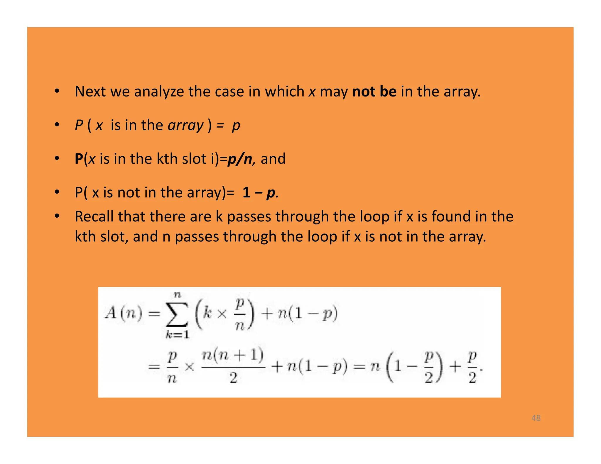
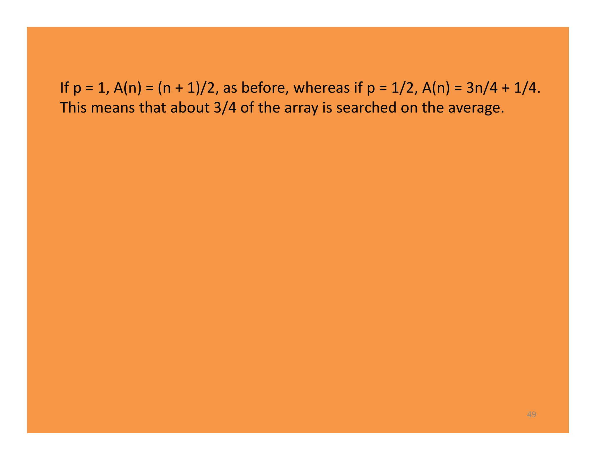
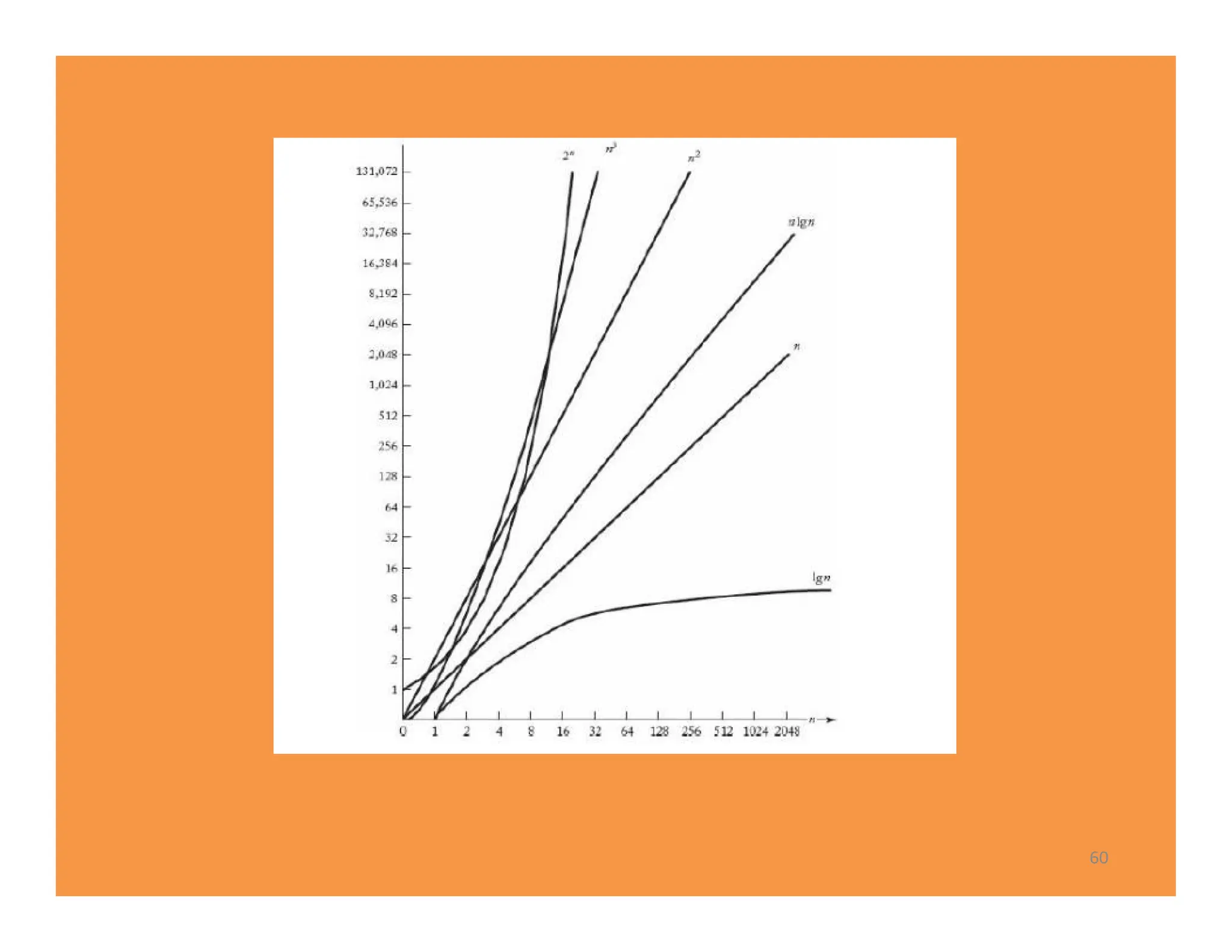
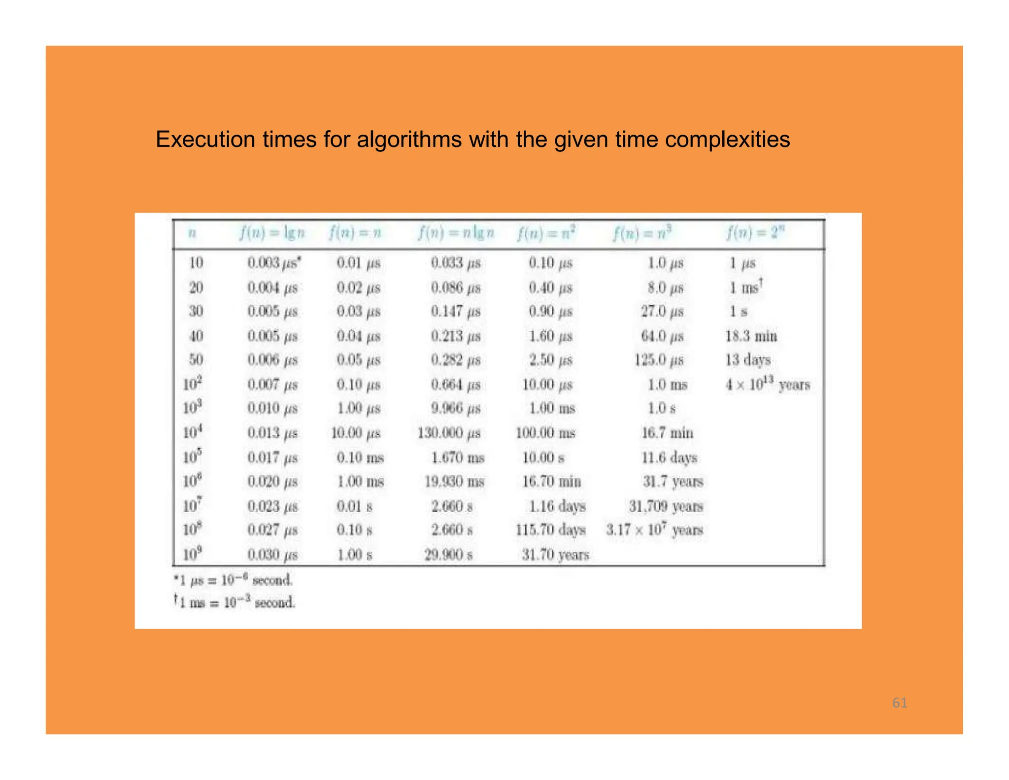
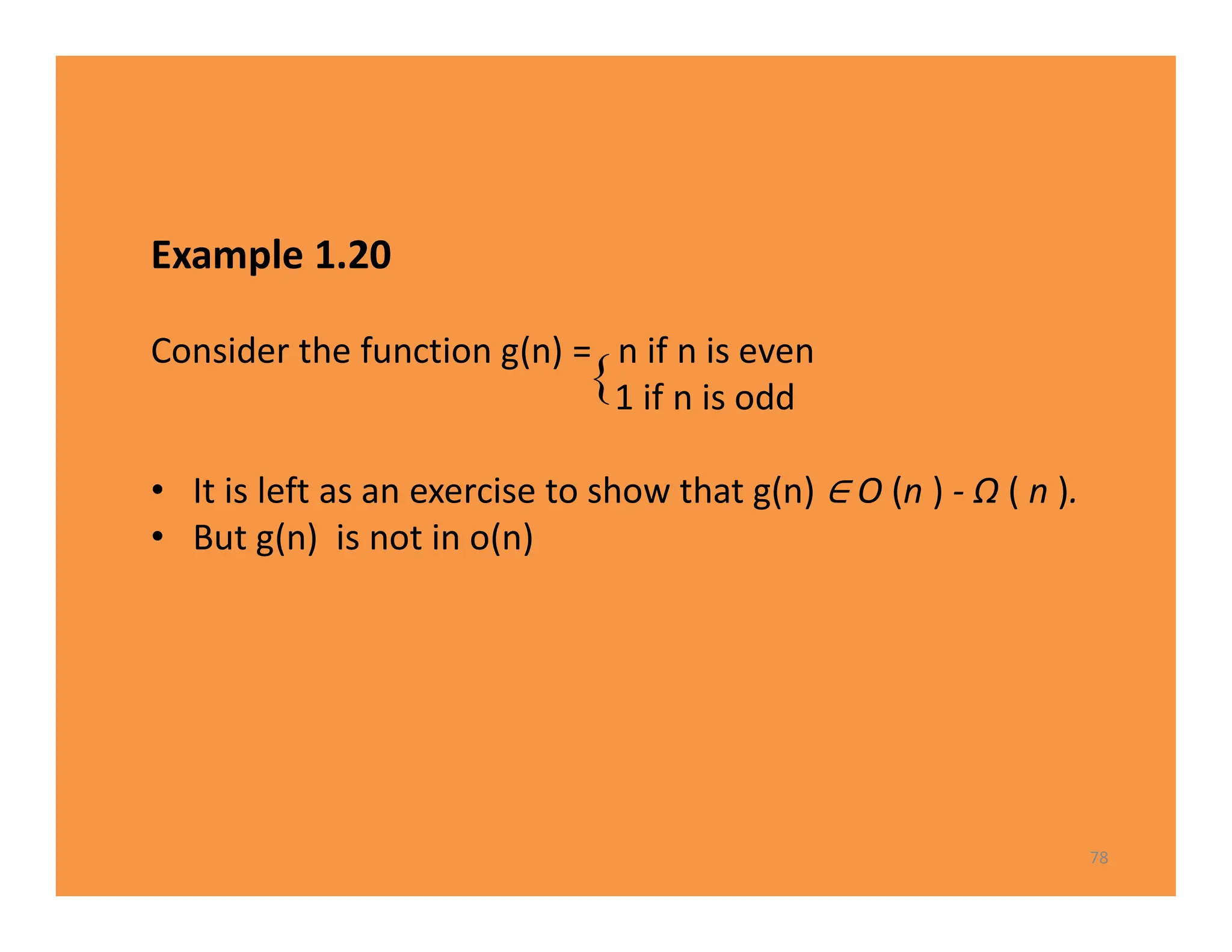
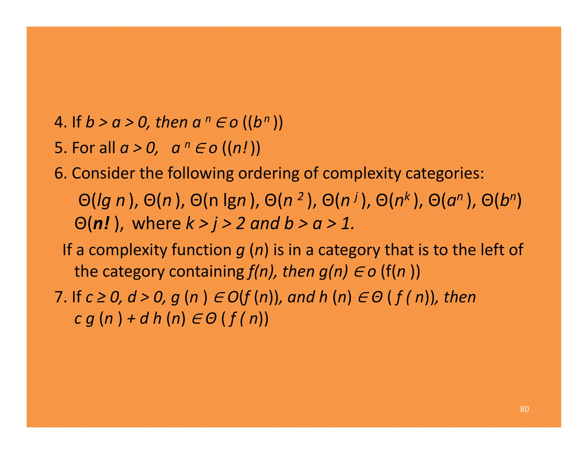
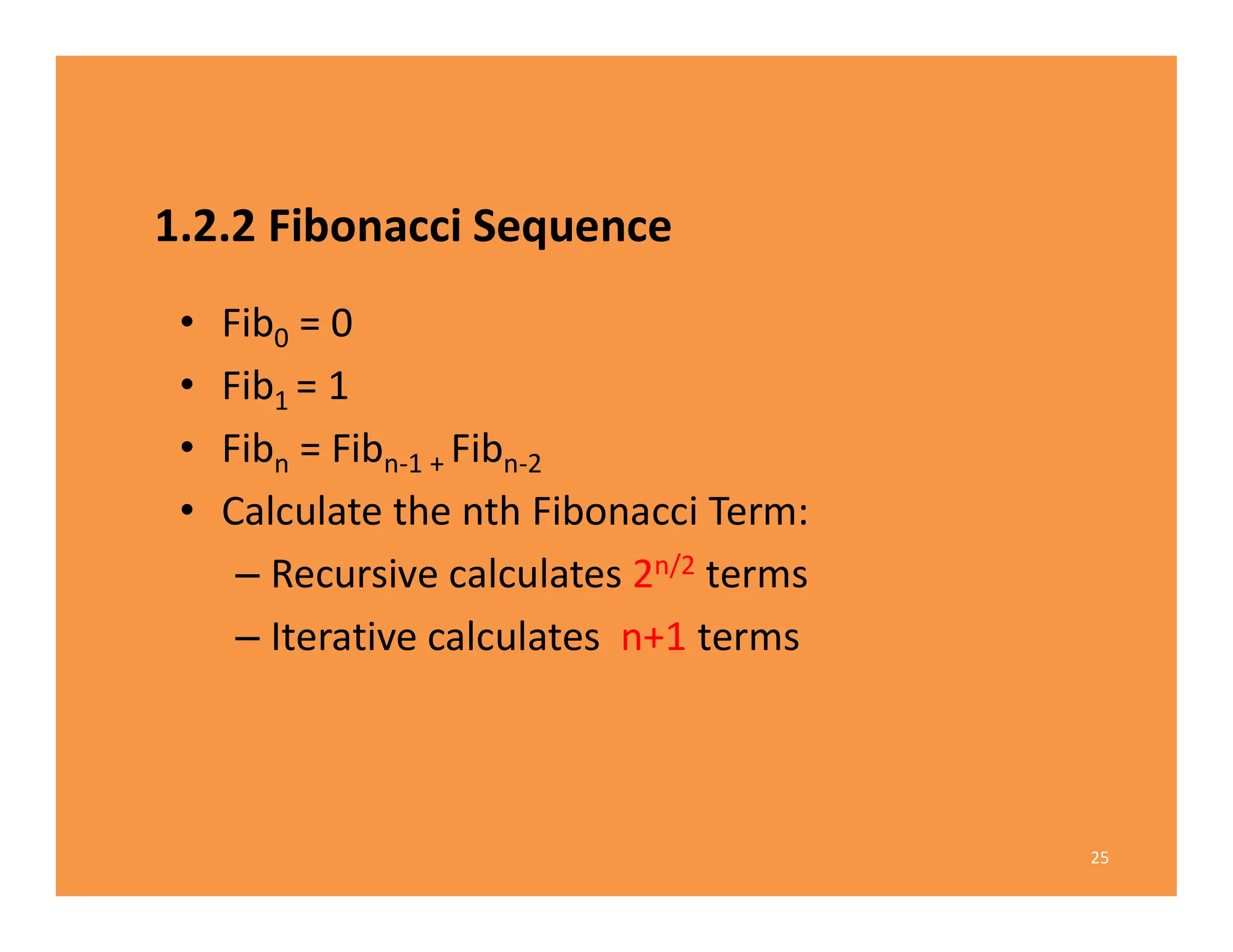
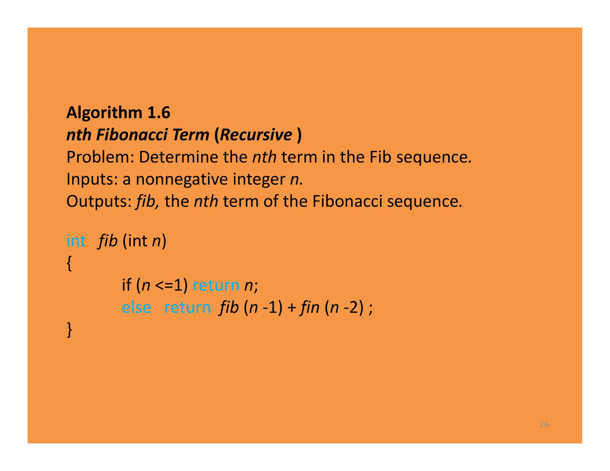
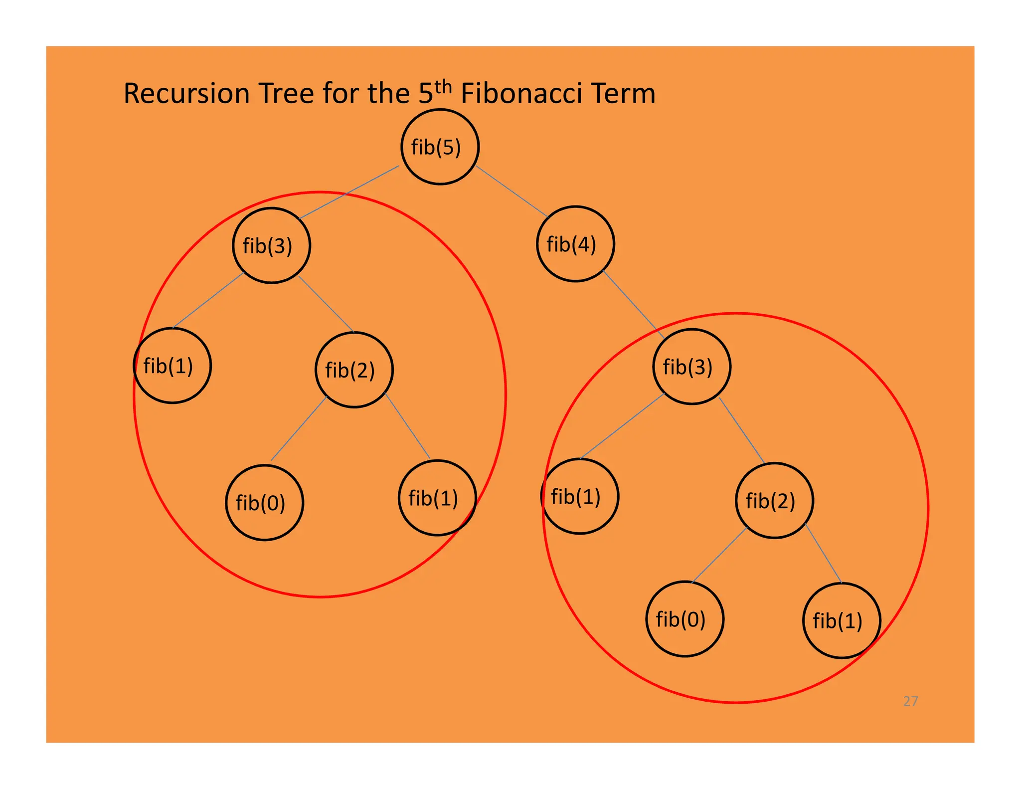
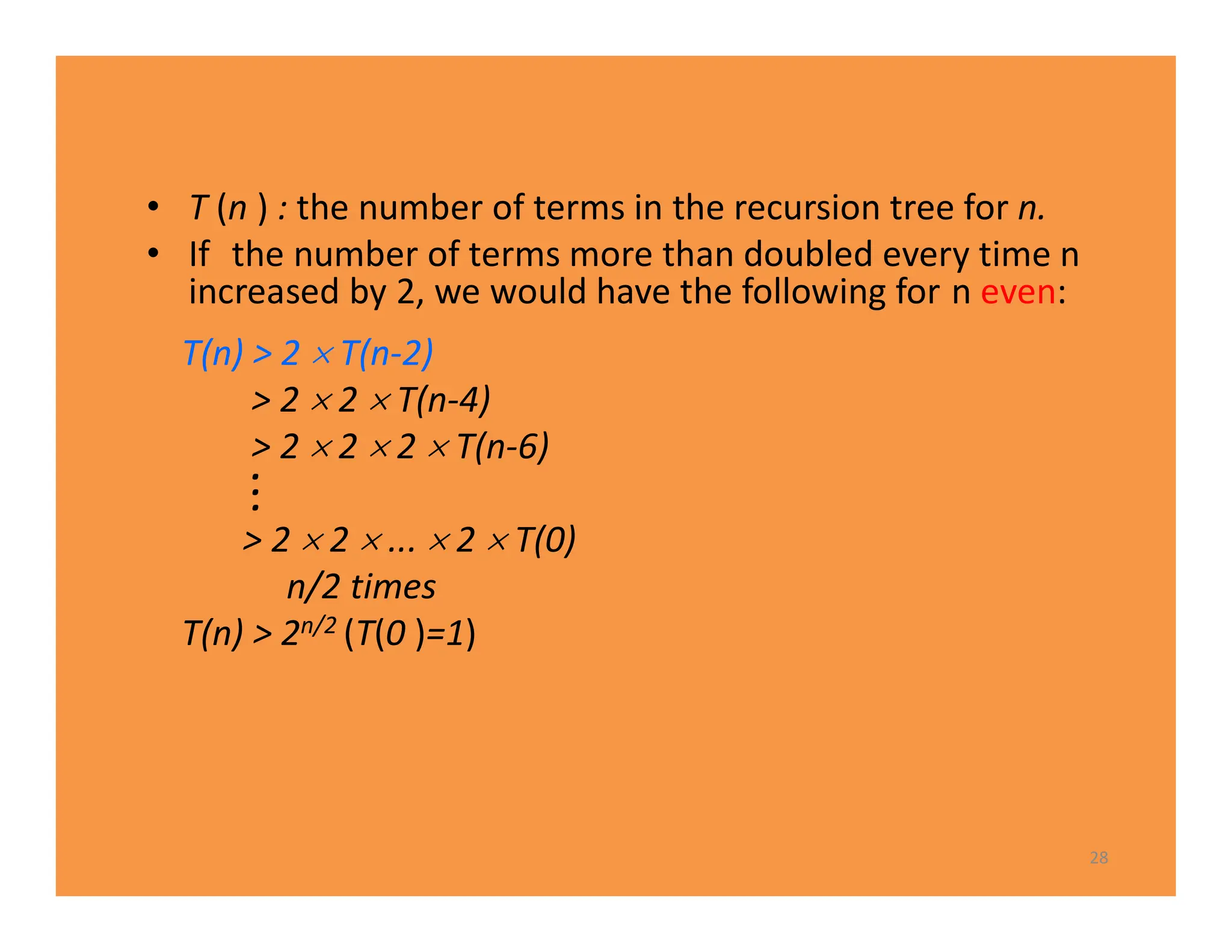
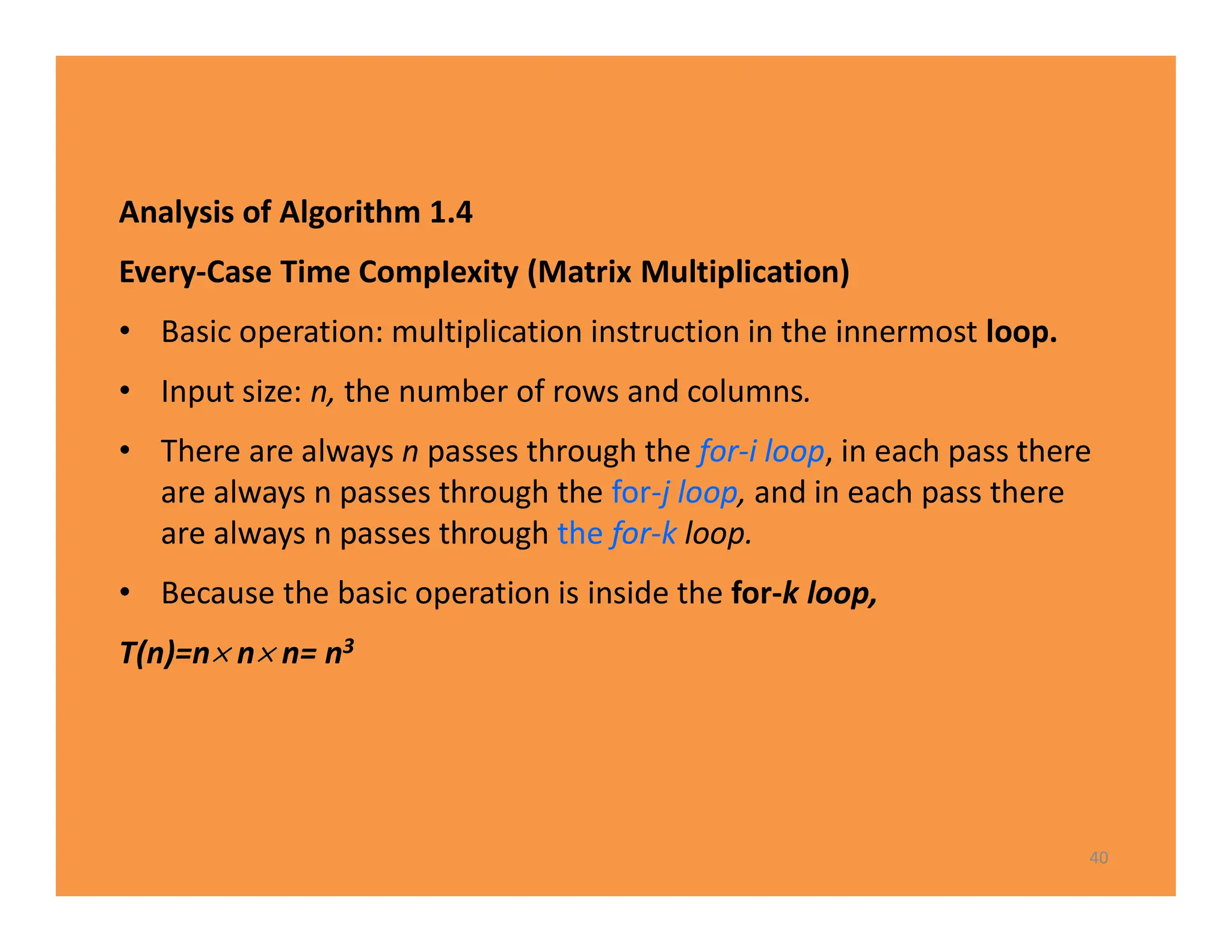
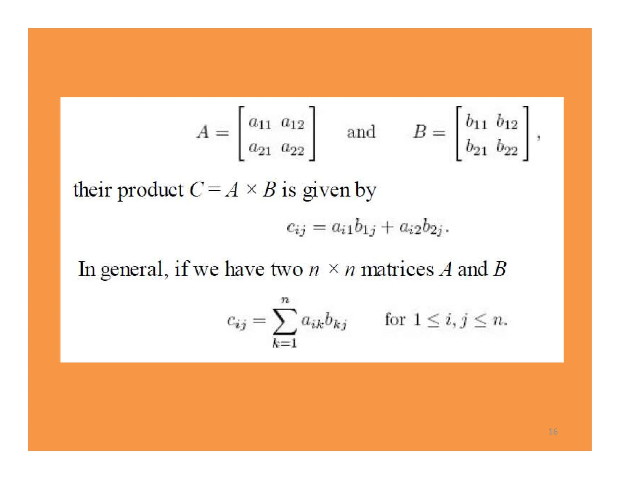
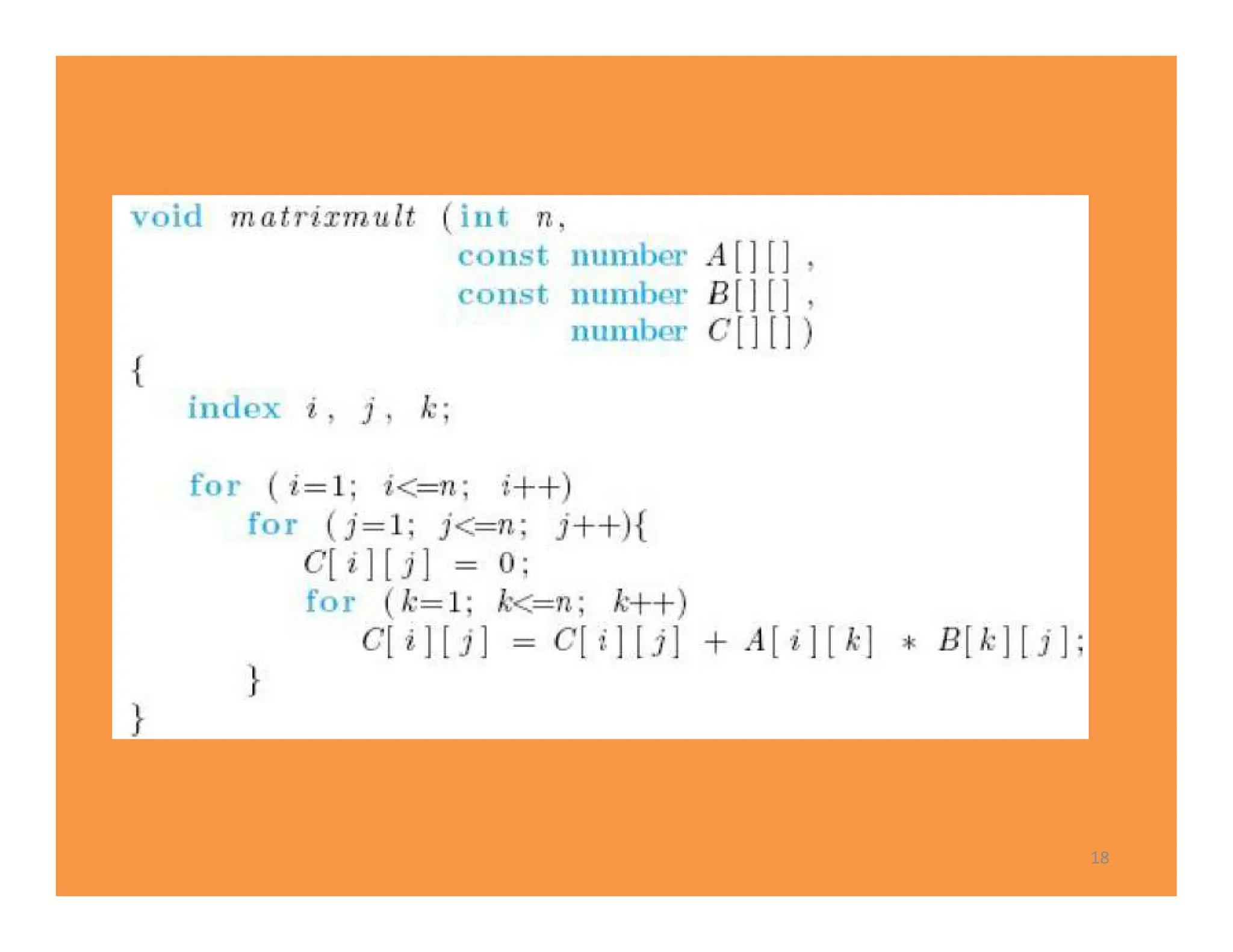
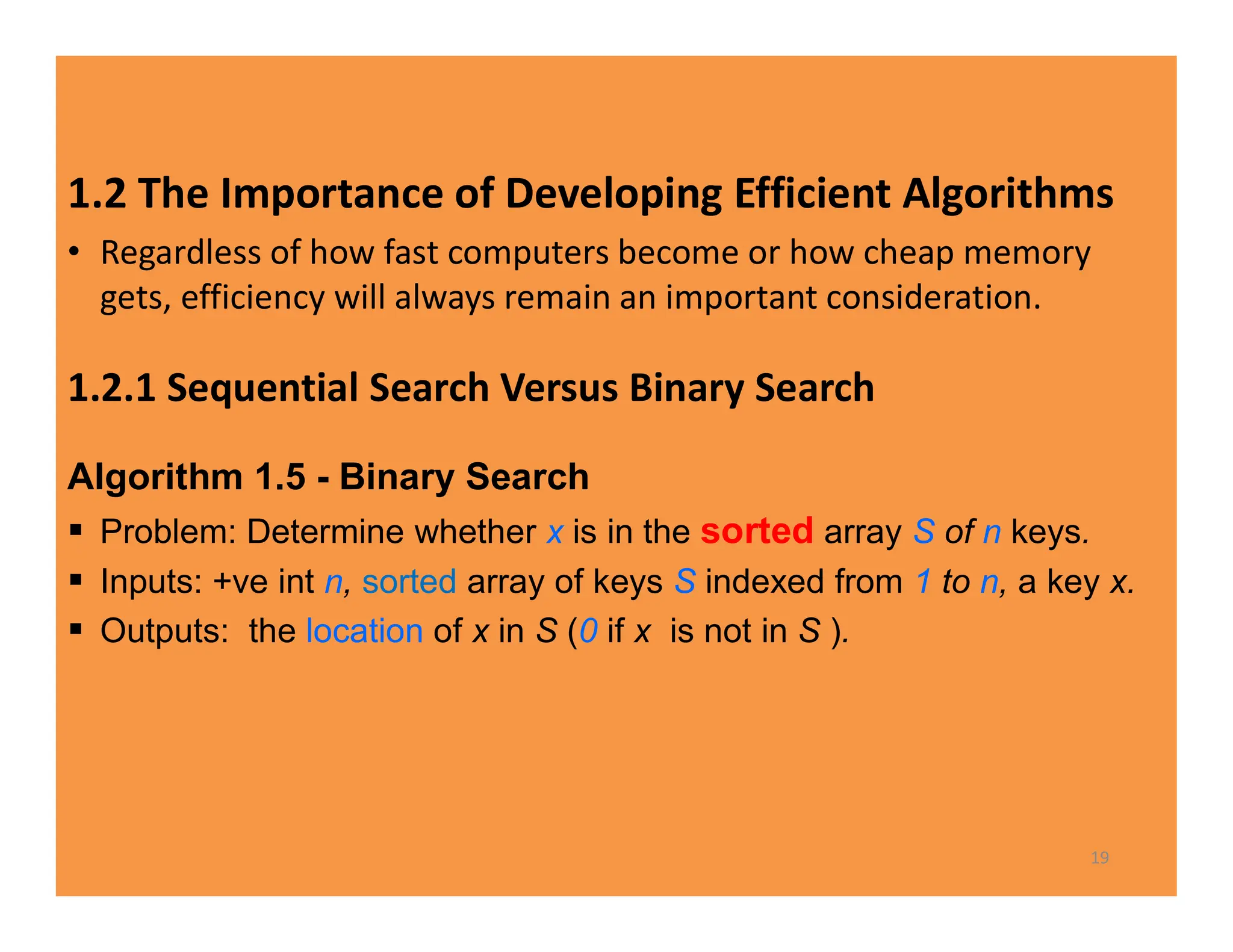
The document discusses algorithms and their analysis. It defines an algorithm as a step-by-step procedure for solving a problem and analyzes the time complexity of various algorithms. Key points made include: 1) Algorithms are analyzed based on how many times their basic operation is performed as a function of input size n. 2) Common time complexities include O(n) for sequential search, O(n^3) for matrix multiplication, and O(log n) for binary search. 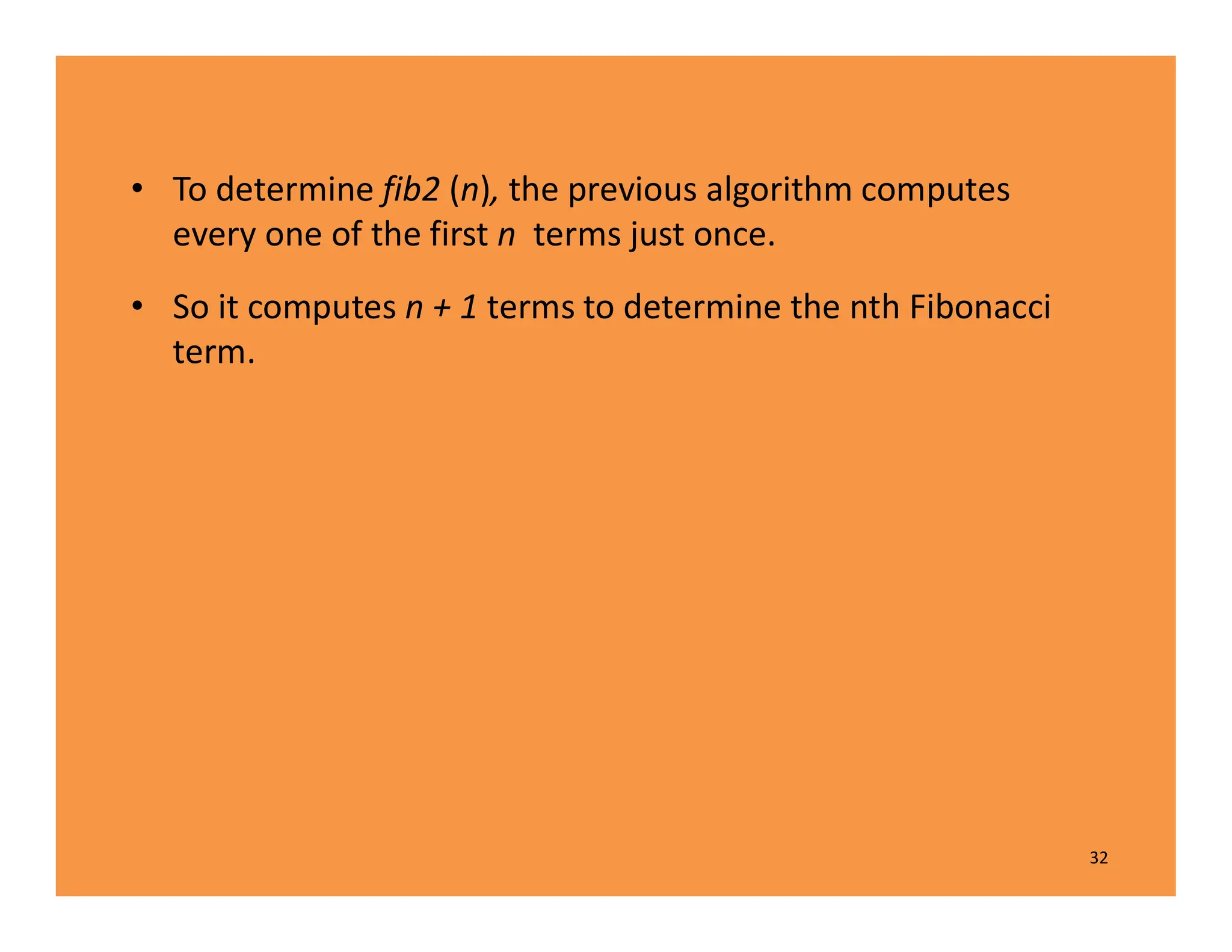3) Recursive algorithms like fibonacci are inefficient and iterative versions improve performance by storing previously computed values.

1. Algorithms:
Efficiency, Analysis, and Order
Chapter 1
1

2. Objectives
• Define an algorithm
• Define growth rate of an algorithm as a function of
input size
• Define Worst case, average case, and best case
complexity analysis of algorithms
• Classify functions based on growth rate
• Define growth rates: Big O, Theta, and Omega
2

3. Problem?
1.1 Algorithms
• Applying a technique to a problem results in a step-by-
step procedure for solving the problem. This step-by-
step procedure is called an algorithm.
• A computer program is composed of individual
modules, that solve specific tasks.
• These tasks are called problems.
3

4. Example 1.1
• Sort a list S of n numbers in nondecreasing order.
• Answer? Numbers in sorted sequence
Example 1.2
• Input : Array S, size n
• Determine whether x  S
• Answer? Yes or No
• Sequential Search: n operations
• Binary Search: lg n + 1 operations
4

5. • Parameters : A problem may contain variables that are not
assigned specific values in the statement of the problem.
• Example 1.1 : two parameters: S and n .
• Example 1.2 : three parameters: S, n, and x.
• It is not necessary in these two examples to make n one of the
parameters because its value is uniquely determined by S.
5

6. • Because a problem contains parameters, it represents a class of
problems, one for each assignment of values to the parameters.
• instance of the problem : Each specific assignment of values to the
parameters
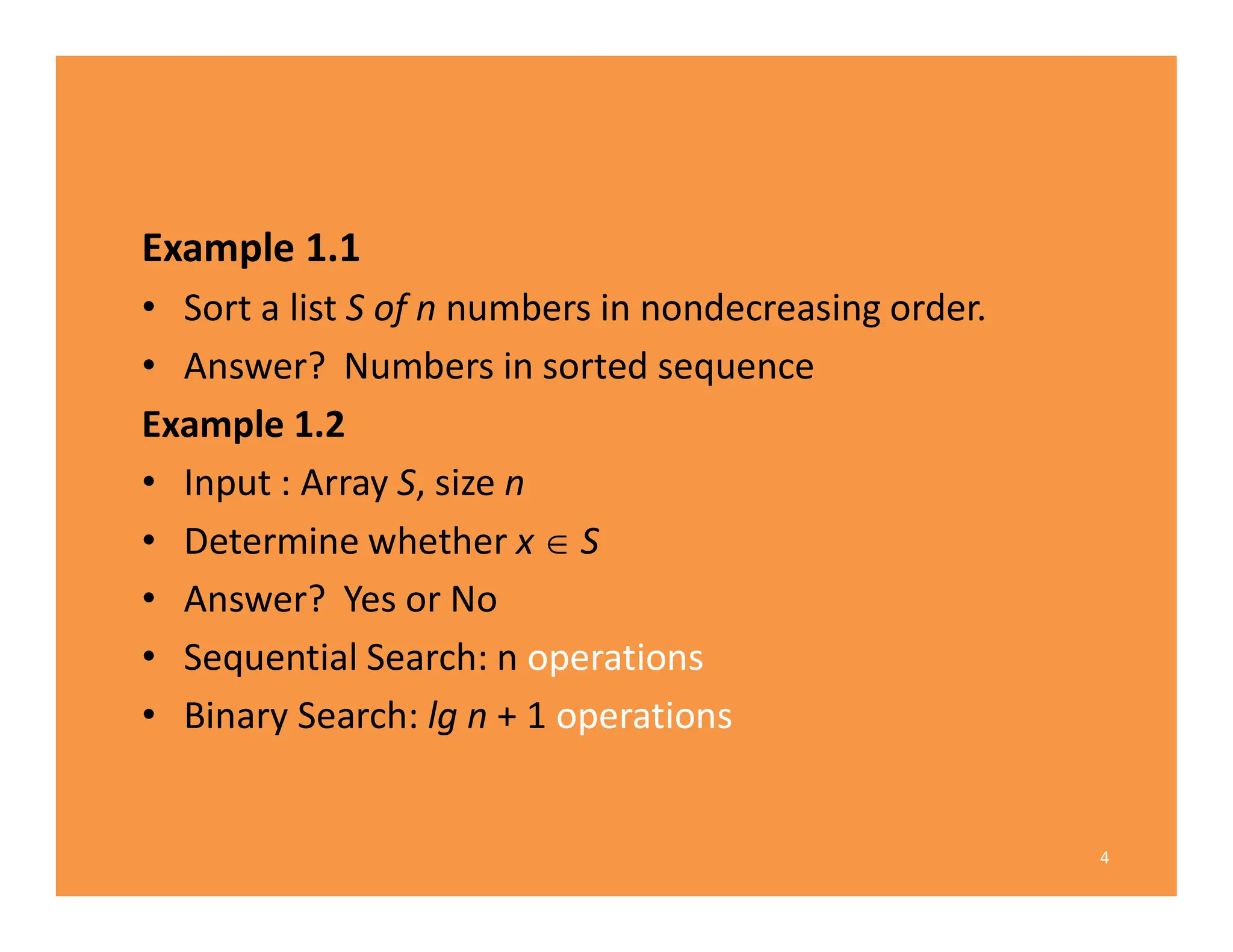
Example 1.3
• An instance of the problem (sorting) in Example 1.1 is
• S = [10, 7, 11, 5, 13, 8] and n=6
Example 1.4
• An instance of the problem (searching) in Example 1.2 is
• S = [10, 7, 11, 5, 13, 8] and n=6 and x=5
The solution to this instance is, “yes, x is in S.”
6

7. Algorithm 1.1 - Sequential Search
• Problem: Is x  S of n keys?
• Inputs (parameters): n, S ( from 1 to n), and x.
• Outputs: the location of x in S (0 if x is not in S ).
7
void seqsearch (int n, const keytype S[ ],
keytype x, index& location )
{
location = 1;
while ( location <= n && S [ location ] != x )
location++;
if (location > n )
location = 0;
}

8. pseudocode
• We can declare
Example
void example (int n)
{
keytype S[2..n];
.
.
.
}
8

9. • Sometimes we use the following nonstandard control
structure:
repeat (n times) { . . . }
9
• We can use mathematical expressions or English-like
descriptions
if ( low  x  high )
rather than
if ( low <= x && x <= high ) { }
Exchange x and y rather than t = x;
x = y;
y = t;

10. • We use the following, which also are not predefined C++ data
types:
10
Data Type Meaning
index A variable used as a index
number A variable could be int or float
bool A variable can take “true” or “false”

11. • function : the algorithm returns a value
• Otherwise, we write the algorithm as a void function and use
reference parameters to return values.
• the defined data type keytype for the items means the items are
from any ordered set.
• If the parameter is not an array, it is declared with an ampersand
(&) . This means that the parameter contains a value
returned by the algorithm.
• we use const to indicate that the array does not contain values
returned by the algorithm.
11

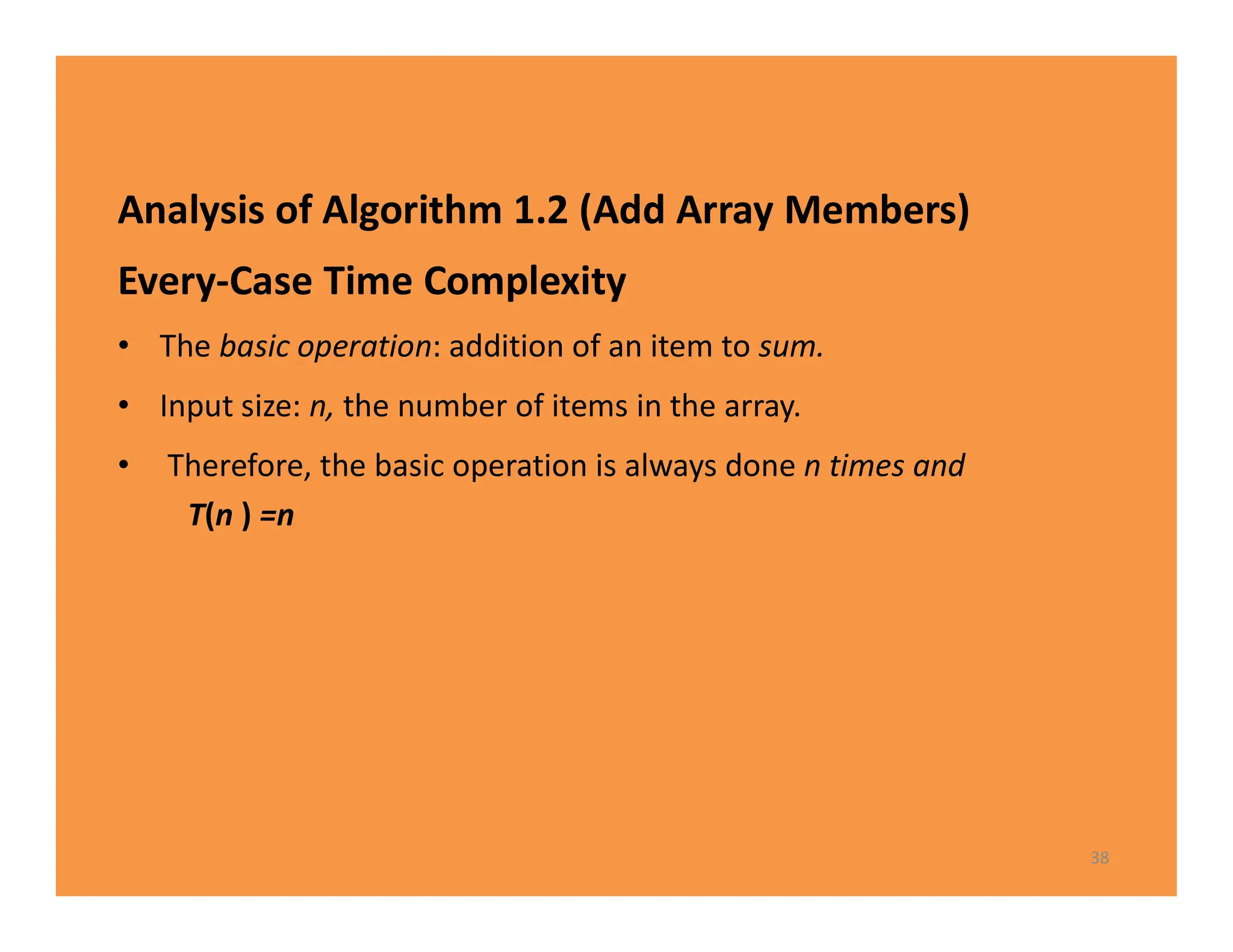
12. Algorithm 1.2 Add Array Members
• Inputs: +ve integer n, array of numbers S indexed from 1 to n.
• Outputs: sum, the sum of the numbers in S.
12
number sum (int n, const number S [ ] )
{
index i;
number result;
result = 0;
for ( i = 1; i <= n; i++ )
result = result + S [ i ];
return result ;
}

13. Exchange Sort
• Exchange Sort works by comparing the number in the ith slot
with the numbers in the (i + 1)st through nth slots.
• Whenever a number in a given slot is found to be smaller than
the one in the ith slot, the two numbers are exchanged.
• In this way, the smallest number ends up in the first slot after
the first pass through for-i loop, the second-smallest number
ends up in the secondslot after the second pass, and so on.
13

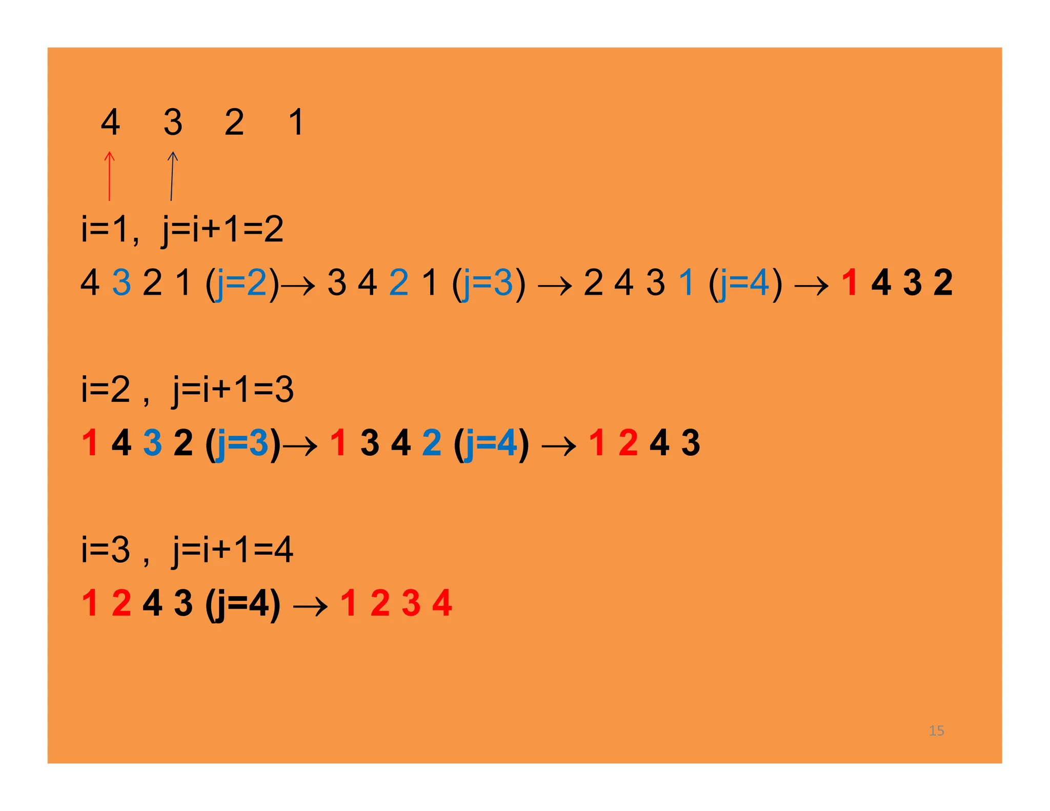
14. Algorithm 1.3 Exchange Sort
• Problem: Sort n keys in nondecreasing order.
• Inputs: +ve integer n, array of keys S indexed from 1 to n.
• Outputs: the array S containing the keys in nondecreasing order.
14
void exchangesort (int n, keytype S [ ] )
{
index i , j;
for ( i = 1; i <= n -1; i ++ )
for ( j = i + 1; j <= n; j++ )
if ( S[ j ] < S[ i ] )
exchange S [ i ] and S[ j ] ;
}

15. 4 3 2 1
i=1, j=i+1=2
4 3 2 1 (j=2) 3 4 2 1 (j=3)  2 4 3 1 (j=4)  1 4 3 2
i=2 , j=i+1=3
1 4 3 2 (j=3) 1 3 4 2 (j=4)  1 2 4 3
i=3 , j=i+1=4
1 2 4 3 (j=4)  1 2 3 4
15

16. Matrix multiplication
16

17. Algorithm 1.4
Matrix Multiplication
• Problem: Find the product of two n × n matrices.
• Inputs: a +ve integer n, two-dimensional arrays of numbers A
and B, rows and columns indexed from 1 to n.
• Outputs: a two-dimensional array of numbers C, - its rows and
columns indexed from 1 to n, containing the product of A and B.
17

18. 18

19. 1.2 The Importance of Developing Efficient Algorithms
• Regardless of how fast computers become or how cheap memory
gets, efficiency will always remain an important consideration.
1.2.1 Sequential Search Versus Binary Search
Algorithm 1.5 - Binary Search
 Problem: Determine whether x is in the sorted array S of n keys.
 Inputs: +ve int n, sorted array of keys S indexed from 1 to n, a key x.
 Outputs: the location of x in S (0 if x is not in S ).
19

20. 20
void binsearch ( int n, const keytype S [ ],
keytype x, index& location )
{
index low , high, mid;
low = 1; , high = n ;
location = 0 ;
while (low <= high && location ==0){
mid= ( low + high )/2  ;
if ( x == S [ mid ] )
location = mid;
else if ( x < S [ mid ] )
high = mid - 1;
else
low = mid + 1;
}
}

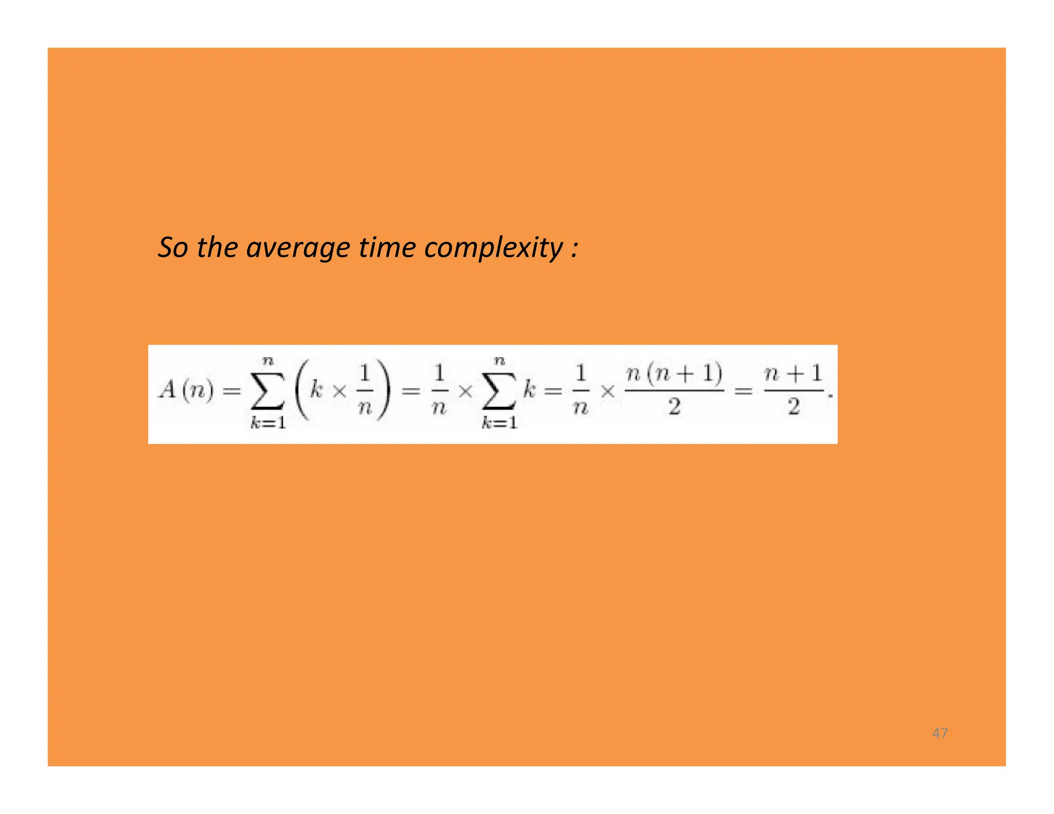
21. • We consider the number of comparisons done by each algorithm.
• Sequential Search : n comparisons if x is not in the array .
• There are two comparisons of x with S [mid ] in each pass through
the while loop.
• In an efficient assembler language implementation of the
algorithm, x would be compared with S[mid] only .
• This means that there would be only one comparison of x with
S[mid] in each pass through the while loop. We will assume the
algorithm is implemented in this manner.
21

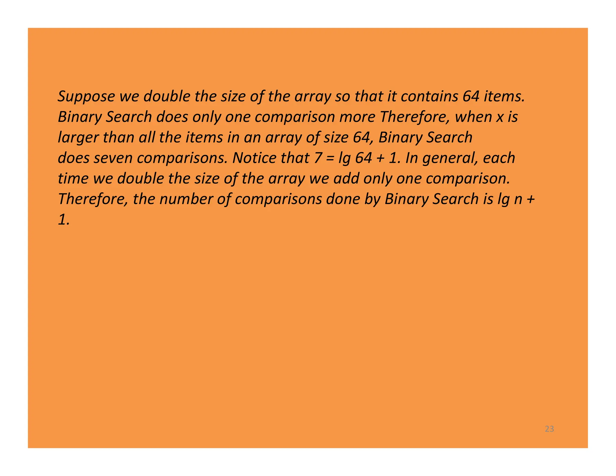
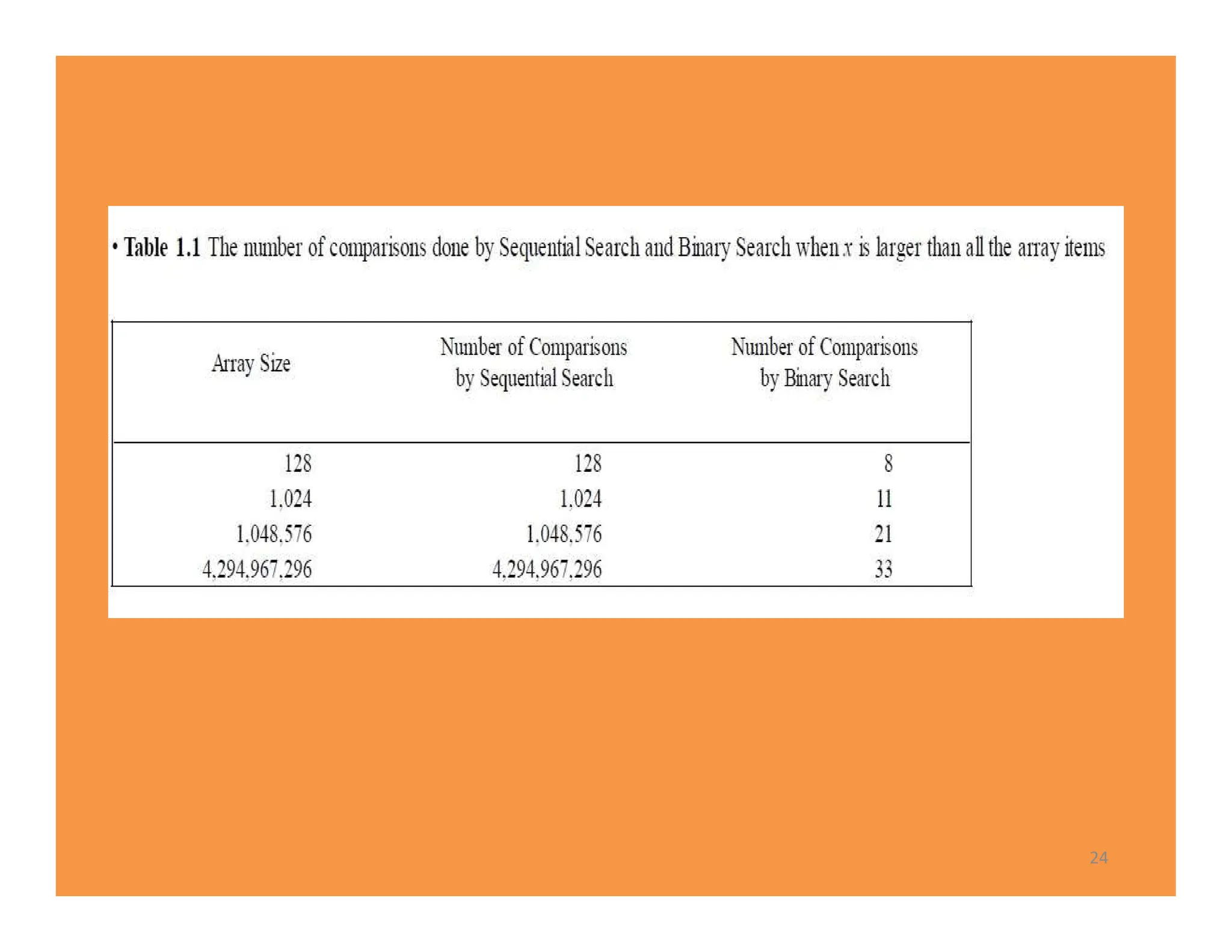
22. • n=32, Assume that x is larger than all the array
• The algorithm does six comparisons when x is larger than all the
items in an array of size 32.
• low=1, high=32, mid=  low+ high/2 =16, high=32
• low=17, high=32, mid=  (17+ 32)/2 =24
• low=25, high=32, mid=  (25+ 3 )/ 2 =28
• The algorithm does six comparisons
• …….
S[16] S[24] S[28] S[30] S[31] S[32]
     
1st 2nd 3rd 4th 5th 6th
Notice that 6 =1+ lg 32
22

23. 23
Suppose we double the size of the array so that it contains 64 items.
Binary Search does only one comparison more Therefore, when x is
larger than all the items in an array of size 64, Binary Search
does seven comparisons. Notice that 7 = lg 64 + 1. In general, each
time we double the size of the array we add only one comparison.
Therefore, the number of comparisons done by Binary Search is lg n +
1.

24. 24

25. 1.2.2 Fibonacci Sequence
• Fib0 = 0
• Fib1 = 1
• Fibn = Fibn-1 + Fibn-2
• Calculate the nth Fibonacci Term:
– Recursive calculates 2n/2 terms
– Iterative calculates n+1 terms
25

26. Algorithm 1.6
nth Fibonacci Term (Recursive )
Problem: Determine the nth term in the Fib sequence.
Inputs: a nonnegative integer n.
Outputs: fib, the nth term of the Fibonacci sequence.
26
int fib (int n)
{
if (n <=1) return n;
else return fib (n -1) + fin (n -2) ;
}

27. 27
Recursion Tree for the 5th Fibonacci Term
fib(5)
fib(3)
fib(1) fib(2)
fib(0) fib(1)
fib(3)
fib(1) fib(2)
fib(0) fib(1)
fib(4)

28. • T (n ) : the number of terms in the recursion tree for n.
• If the number of terms more than doubled every time n
increased by 2, we would have the following for n even:
T(n) > 2  T(n-2)
> 2  2  T(n-4)
> 2  2  2  T(n-6)
.
.
.
> 2  2  ...  2  T(0)
n/2 times
T(n) > 2n/2 (T(0 )=1)
28

29. Theorem 1.1
If T (n ) is the number of terms in the recursion tree
corresponding to Algorithm 1.6, then, for n ≥ 2,
T(n) > 2 n/2
Proof : See page 32(by induction on n)
29

30. 30
let’s develop an efficient algorithm for computing the nth
Fibonacci term. Recall that the problem with the recursive
algorithm is that the same value is computed over and over. As
Figure 1.2 shows, fib(2) is computed three times in determining
fib(5). If when computing a value, we save it in an array, then
whenever we need it later we do not need to recompute it.

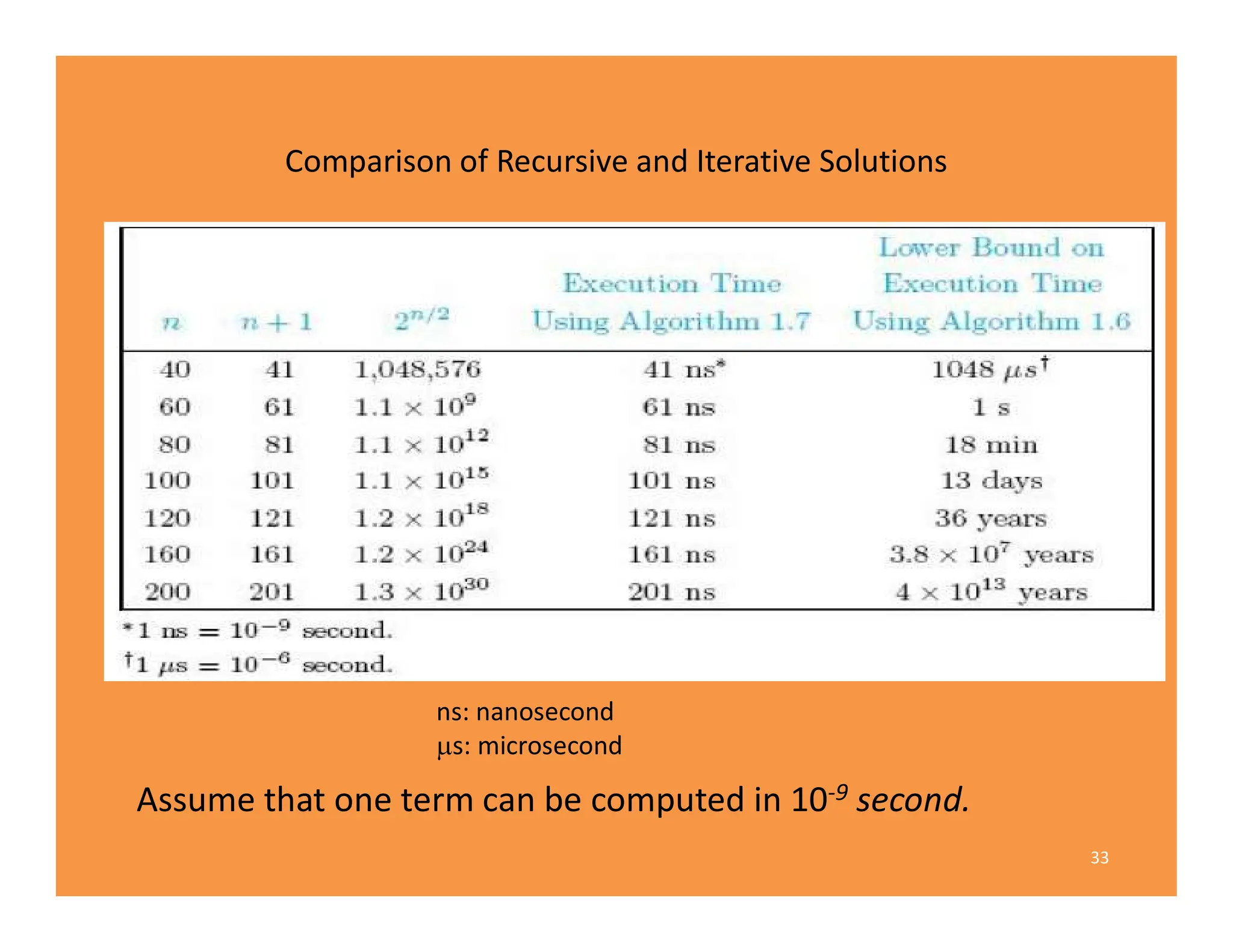
31. Algorithm 1.7
nth Fibonacci Term (Iterative)
Problem: ....
Inputs: n.
Outputs: fib2, the nth term in the Fibonacci sequence.
31
int fib2 (int n)
{
index i;
int f [0 . . n];
f [0] = 0;
if (n > 0) {
f [1] = 1;
for ( i = 2; i <= n; i ++ )
f [ i ] = f [i - 1] + f [i - 2] ;
};
return f [ n ] ;
}

32. • To determine fib2 (n), the previous algorithm computes
every one of the first n terms just once.
• So it computes n + 1 terms to determine the nth Fibonacci
term.
32

33. Comparison of Recursive and Iterative Solutions
33
ns: nanosecond
s: microsecond
Assume that one term can be computed in 10-9 second.

34. 1.3 Analysis of Algorithms
• To determine how efficiently an algorithm solves a problem.
1.3.1 Complexity Analysis
• When analyzing the efficiency of an algorithm:
o we do not count every instruction executed ( depends on the
programming language and the programmer).
• We want a measure that is independent of the computer.
34

35. • Define Basic Operation (instruction or group of instructions)
• Time complexity analysis of an algorithm: how many times the
basic operation is done as a function of the size of the input.
• Consider Algorithms Sequential Search, Add Array Members,
Exchange Sort, and Binary Search: n, the number of items in the
array, is a simple measure of the size of the input. Therefore, we
can call n the input size.
• Algorithm Matrix Multiplication, n, is a simple measure of the
size of the input. Therefore, we can again call n the input size.
35

36. • In Algorithms 1.6 (nth Fibonacci Term, Recursive) n is the input; it is
not the size of the input.
• For this algorithm, a reasonable measure of the size of the input is
the number of symbols used to encode n.
• There is no hard-and-fast rule for choosing the basic operation. It is
largely a matter of judgment and experience.
• We ordinarily do not include the instructions that make up the
control structure (we do not include the instructions that increment
and compare the index in order to control the passes through the
while loop)
36

37. • Sometimes complexity depends on instance.
• Consider Sequential Search. If x is the first item in the array, the
basic operation is done once, whereas if x is not in the array, it is
done n times.
• T (n ) (every-case time complexity of the algorithm) : exists when
the basic operation is always done the same number of times for
every instance of size n.
37

38. Analysis of Algorithm 1.2 (Add Array Members)
Every-Case Time Complexity
• The basic operation: addition of an item to sum.
• Input size: n, the number of items in the array.
• Therefore, the basic operation is always done n times and
T(n ) =n
38

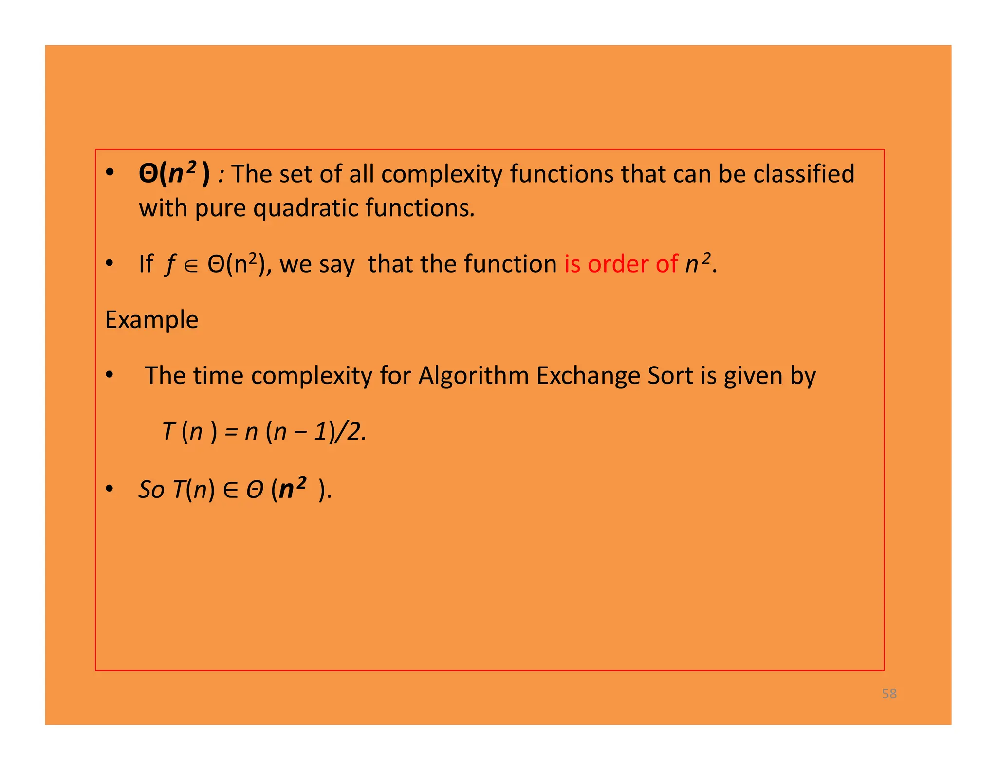
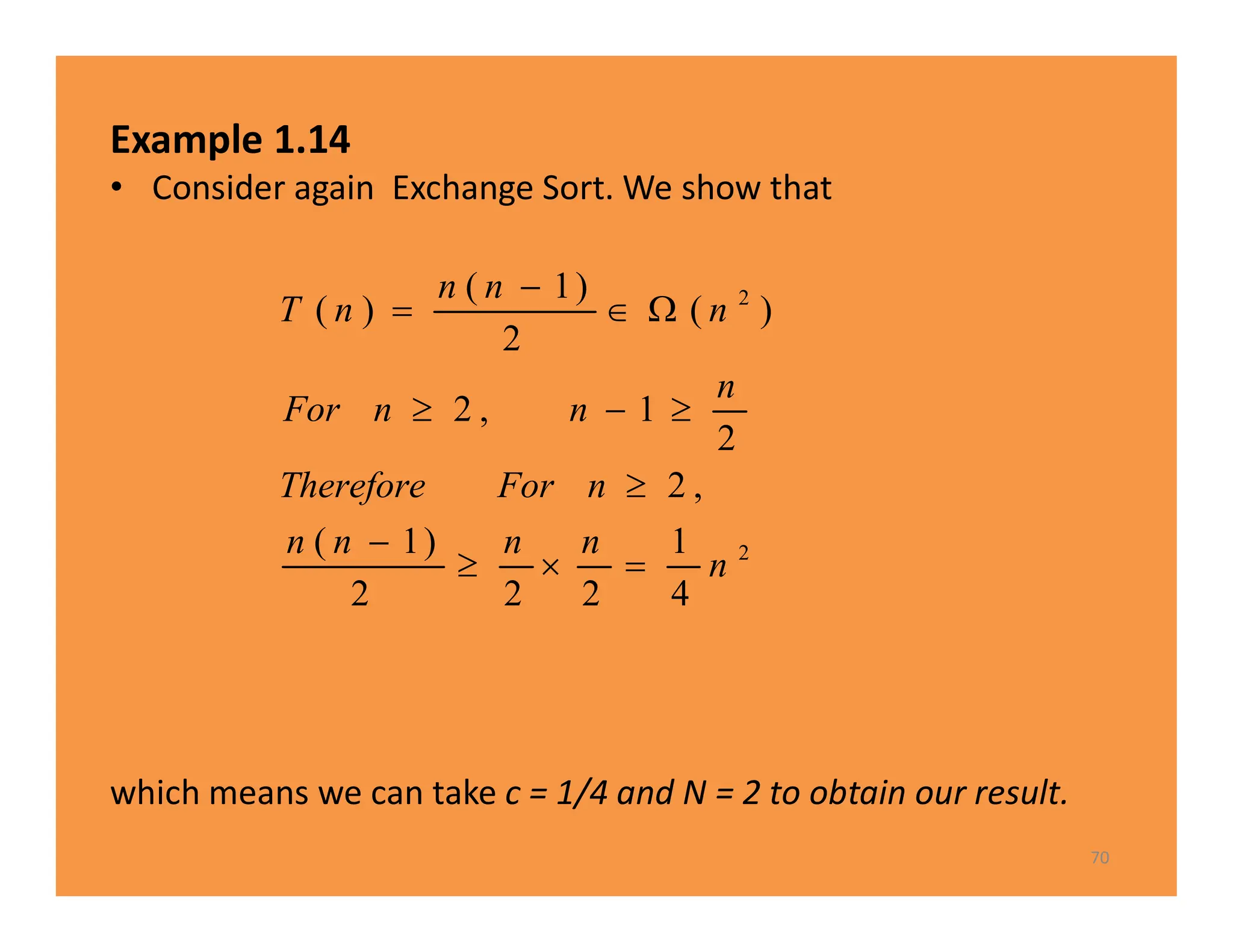
39. Analysis of Algorithm 1.3
Every-Case Time CompIexity (Exchange Sort)
• Basic operation: the comparison of S [ j ] with S [i ].
• Input size: n, the number of items to be sorted.
• there are always n − 1 passes through the for-i loop.
– first pass, there are n − 1 passes through the for-j loop,
– second pass there are n − 2 passes through the for-j loop,
– third pass there are n−3 passes through the for-j loop, … ,
– last pass, there is one pass through the for-j loop.
– Therefore, total number of passes is given by
T(n)=(n-1)+(n-2)+...+1=(n-1) *n/2
39

40. Analysis of Algorithm 1.4
Every-Case Time CompIexity (Matrix Multiplication)
• Basic operation: multiplication instruction in the innermost loop.
• Input size: n, the number of rows and columns.
• There are always n passes through the for-i loop, in each pass there
are always n passes through the for-j loop, and in each pass there
are always n passes through the for-k loop.
• Because the basic operation is inside the for-k loop,
T(n)=n n n= n3
40

41. 41
If the algorithm does not have an every-case time complexity. This does
not mean that we cannot analyze such algorithms,
• Worst-case time complexity W(n)
• Average-case time complexity A(n)
• Best-case time complexity B(n)

42. • The worst-case time complexity: W (n ) is the maximum number of
times the algorithm will ever do its basic operation for an input size
of n.
• T (n ) (every-case time complexity of the algorithm) : exists when
the basic operation is always done the same number of times for
every instance of size n.
• If T (n ) exists, then clearly W (n ) = T (n ).
• The following is an analysis of W (n) in a case in which T (n) does not
exist.
• In sequential search algorithm if x is the first element in the array we
need only one comparison operation.
42

43. • The basic operation is done n times, if x is the last item in
the array or if x is not in the array.
• Therefore, W(n) = n
43

44. Average
• A (n ) is the average (expected value) of the no of times the
algorithm does the basic operation for an input size of n
• A (n) is called the average-case time complexity of the
algorithm.
• If T (n) exists, then
A (n ) = T (n ).
44

45. • To compute A(n), we need to assign probabilities to all possible
inputs of size n.
• Consider Algorithm 1.1.
• We will assume that if x is in the array, it is equally likely to be in
any of the array slots, and the items in S are all distinct
• It is reasonable to assign equal probabilities to all array slots.
45

46. 1.3 Analysis of Algorithms
Analysis of Algorithm 1.1 (Sequential Search)
• Average-Case Time Complexity
• Basic operation: comparison with x.
• Input size: n
• First, assume that x is in S, where the items in S are all distinct
• For 1 ≤ k ≤ n, the probability that x is in the kth array slot is 1/n.
• If x is in the kth array slot, the number of times the basic
operation is done to locate x) is k.
46

47. 47
So the average time complexity :

48. • Next we analyze the case in which x may not be in the array.
• P ( x is in the array ) = p
• P(x is in the kth slot i)=p/n, and
• P( x is not in the array)= 1 − p.
• Recall that there are k passes through the loop if x is found in the
kth slot, and n passes through the loop if x is not in the array.
48

49. 49
If p = 1, A(n) = (n + 1)/2, as before, whereas if p = 1/2, A(n) = 3n/4 + 1/4.
This means that about 3/4 of the array is searched on the average.

50. • B (n) is defined as the minimum number of times the algorithm
will ever do its basic operation for an input size of n.
• B (n) is called the best-case time complexity of the algorithm,
• if T(n) exists, then B (n ) = T (n ).
• Because n ≥ 1, there must be at least one pass through
Therefore, B(n)=1
50

51. • A complexity function can be any function that maps the
positive integers to the nonnegative reals
• Complexity function: a function
f: N+  R≥0
Examples
f (n ) = n3
g (n )=lg n
51

52. Analysis of Correctness
• we can analyze the correctness of an algorithm
by developing a proof that the algorithm actually
does what it is supposed to do. Although we will
often informally show that our algorithms are
correct and will sometimes prove that they are,
you should.
• see Dijkstra (1976), Gries (1981), or Kingston
(1990) for a comprehensive treatment of
correctness.
52

53. 1.4 Order
• An algorithm with a time complexity of n is more
efficient than one with a time complexity of n 2 for
sufficiently large values of n.
• Consider two algorithms A, and B for the same problem
such that
– A: every-case time complexities 100 n
– B: every-case time complexities 0.01 n 2
• The first algorithm will be more efficient if
0.01n2 > 100 n  n > 10000
53

54. 54
0
500000
1000000
1500000
2000000
2500000
3000000
3500000
4000000
4500000
0 2000 4000 6000 8000 10000 12000 14000 16000 18000 20000
100 n
0.01 n 2

55. • linear-time algorithms : time complexities are linear in
the input size n(n, 100n, 0.7n).
• n2 and 0.01n2 : quadratic-time algorithms .
• Any linear-time algorithm is more efficient than any
quadratic-time algorithm.
55

56. 1.4.1 An Introduction to Order
• 5n2 and 5 n2 + 100 : pure quadratic functions (no linear term),
• 0.1 n2 + n + 100 : a complete quadratic function
• Complete quadratic function can be classified with the pure
quadratic functions.
• We should always be able to throw away low-order terms
when classifying complexity functions.
• For example, it seems that we should be able to classify
0.1 n3 + 10n2 + 5n + 25 with pure cubic functions.
56

57. 57
Table 1.3 shows that the quadratic term dominates this function.

58. • Θ(n2 ) : The set of all complexity functions that can be classified
with pure quadratic functions.
• If f  Θ(n2), we say that the function is order of n2.
Example
• The time complexity for Algorithm Exchange Sort is given by
T (n ) = n (n − 1)/2.
• So T(n) Θ (n2 ).
58

59. • quadratic-time algorithm : the algorithm’s time complexity is in
Θ(n2 ). We also say that the algorithm is Θ(n2 ).
• Exchange Sort is a quadratic-time algorithm.
• Similarly, the set of complexity functions that can be classified
with pure cubic functions is called Θ(n3 ), and functions in that
set are said to be order of n3.
• We will call these sets complexity categories.
• Examples of the most common complexity categories:
Θ(lg n ), Θ(n ), Θ(n lgn ), Θ(n2 ), Θ(n3 ), Θ(2n ),
59

60. 60

61. 61
Execution times for algorithms with the given time complexities

62. 1.4.2 A Rigorous Introduction to Order
Definition
• g (n ) O ( f (n ) ) if :
there exists some positive real constant c and some
nonnegative integer N such that
for all n ≥ N, g (n ) ≤ c  f (n )
• If g (n ) O (f (n )), we say that g (n) is big O of f (n ).
• If g (n) O (n2 ), then eventually g(n) lies beneath some pure
quadratic function c n2 on a graph.
62

63. Example 1.8
• Recall that the time complexity of Algorithm 1.3 (Exchange Sort)
we can take c = 1/2 and N = 0 to conclude that T(n) O (n2 ).
63
2
2
1
2
)
(
2
)
1
(
,
0
2
)
1
(
)
(
n
n
n
n
n
n
for
because
n
n
n
T







64. Example 1.9
• We show that n 2 + 10 n O( n 2 ).
• Because, for n ≥ 0,
n 2 +10 n ≤ n 2 +1 0 n 2 ≤ 11 n 2
• We can also take c = 2 and N = 10
• we can say that eventually g(n) is at least as good
as a pure quadratic function.
• A difficulty students often have with “big O” is
that they erroneously think there is some unique
c and unique N that must be found to show that
one function is “big O” of another. This is not the
case at all.
64

65. 65
• Example: n 2 O(n 2 + 10n). Because, for n ≥ 0,
n 2 n 2
we can take c = 1 and N = 0 to obtain our result.
• Note: the function inside “big O” does not have to be one of the simple
functions
• Example: n O( n 2 ).
• A complexity function need not have a quadratic term to be in O(n2).
• Therefore, any logarithmic or linear complexity function is in O(n2).
any
logarithmic, linear, or quadratic complexity function is in O(n3), and so on.

66. Definition
• f (n ), g (n) : complexity functions.
• g(n) ϵ Ω (f (n )) if there exists some +ve real constant c
and some nonnegative integer N such that,
for all n ≥ N, g(n) ≥ c  f (n)
• If g(n) Ω (f (n )), we say that g (n) is omega of f (n )
66

67. 67
Example:
• 5 n 2 Ω(n 2).
• n 2 + 10n Ω(n 2 ).
N=0 , c=1

68. 68

69. 69

70. Example 1.14
• Consider again Exchange Sort. We show that
which means we can take c = 1/4 and N = 2 to obtain our result.
70
2
2
4
1
2
2
2
)
1
(
,
2
2
1
,
2
)
(
2
)
1
(
)
(
n
n
n
n
n
n
For
Therefore
n
n
n
For
n
n
n
n
T













71. 71
• If a function is in Ω(n 2), then eventually the function
lies above some pure quadratic function on a graph.
For the purposes of analysis, this means that
eventually it is at least as bad as a pure quadratic
function.
• n 3 Ω(n 2) , c = 1 and N = 1.

72. Definition
• For a given complexity function f (n),
Θ(f (n )) = O (f (n ))  Ω (f (n ))
• If g(n) Θ (f (n)), we say that g (n) is order of f(n).
• This means that Θ(f (n)) is the set of complexity functions
g(n) for which there exists some positive real constants c and
d and some nonnegative integer N such that, for all n ≥ N,
c  f (n ) ≤ g(n) ≤ d  f (n)
Example 1.16
Consider again Exchange Sort
T(n) Θ (n2 )
72

73. Example 1.17
Show that n is not in Ω (n 2 ) by using proof by contradiction.
• Assuming that n Ω (n 2 )
• Then there exists some positive constant c and some
nonnegative integer N such that, for n ≥ N, n>= c n 2
1/c >=n, for n ≥ N
• this inequality cannot hold
73

74. Definition
Given f (n), o (f (n )) is the set of all complexity functions g(n )
satisfying the following: For every positive real constant c there
exists a nonnegative integer N such that,
 for all n ≥ N, g (n) ≤ c  f (n)
• This definition says that the bound must hold for every real
positive constant c, which implies that the bound holds for
arbitrarily small c.
• For example, if g(n) o(f(n)), there is an N such that,
for n > N, g(n) ≤ 0.0001 f(n)
74

75. Example 1.18
n  o (n2 )
Example 1.19
• n is not in o(5n). Proof by contradiction to show this, take
c=1/6
75

76. Theorem 1.2
If g ( n) o ( f (n )), then
g(n) O(f(n)) - Ω ( f (n )).
• Proof: Because g ( n) o(f(n)), for every positive real constant c
there exists an N such that, for all n ≥ N,
g ( n) ≤ c  f (n)
which means that the bound certainly holds for some c.
g(n) O(f(n))
To show that g (n ) is not in Ω(f (n)) we use proof by contradiction. If
g(n) Ω(f(n)), then there exists some real constant c > 0 and some
N1 such that, for all n ≥ N1,
g ( n) ≥ c  f (n)
But, because g(n) o(f(n)), there exists some N2 such that, for all n ≥
N2, g ( n)  ≤ c /2  f (n)
Both inequalities would have to hold for all n greater than both N1
and N2. This contradiction proves that g(n) cannot be in Ω(f(n)).
76

77. • You may think that o(f(n)) and O(f(n))−Ω(f(n))
must be the same set. This is not true. There
are unusual functions that are in O(f(n)) −
Ω(f(n)) but that are not in o(f(n)). The
following example illustrates this.
77

78. Example 1.20
Consider the function g(n) = n if n is even
1 if n is odd
• It is left as an exercise to show that g(n) O (n ) - Ω ( n ).
• But g(n) is not in o(n)
78


79. Properties of Order:
1. g (n ) O (f ( n )) if and only if f (n) Ω (g (n )).
2. g (n ) Θ (f (n )) if and only if f (n) Θ (g (n )).
3. If b > 1 and a > 1, then loga n Θ (logb n).
• This implies that all logarithmic complexity functions
are in the same complexity category.
• We will represent this category by Θ(lg n).
79

80. 4. If b > a > 0, then a n o ((bn ))
5. For all a > 0, a n o ((n!))
6. Consider the following ordering of complexity categories:
Θ(lg n), Θ(n), Θ(n lgn), Θ(n 2 ), Θ(n j ), Θ(nk ), Θ(an ), Θ(bn)
Θ(n! ), where k > j > 2 and b > a > 1.
If a complexity function g (n) is in a category that is to the left of
the category containing f(n), then g(n) o (f(n ))
7. If c ≥ 0, d > 0, g (n ) O(f (n)), and h (n) Θ ( f ( n)), then
c g (n ) + d h (n) Θ ( f ( n))
80

81. Example 1.21
• Property 3 : all logarithmic complexity functions are in the
same complexity category.
• For example,
Θ (log4 n )=Θ (lg2 n).
Example 1.23
• Properties 6 and 7 can be used repeatedly. For example, we
can show that 5n + 3 lg n + 10n lg n +7n 2 Θ(n 2 ),
81

82. 82














))
(
(
)
(
))
(
(
)
(
0
0
))
(
(
)
(
)
(
)
(
lim
n
g
o
n
f
implies
n
f
o
n
g
implies
c
if
n
f
n
g
implies
c
n
f
n
g
n
Theorem 1.3
We have

83. 83
Example 1.24
Theorem 1.3 implies that
because
)
(
2
3
2
n
o
n

0
2
1
2
/
lim
lim 3
2





 n
n
n
n
n

84. Example 1.25
• Theorem 1.3 implies that, for b > a > 0, a n o(b n )
Because
Limn∞ a n /b n =0 (The limit is 0 because 0 < a/b < 1 )
From th. 1.3 , a n o(b n )
84