System modeling and simulation full notes by sushma shetty (www.vtulife.com)

1. WWW.VTULIFE.COM 1
Mangalore
System Simulation and
Modelling
8th SEMESTER COMPUTER SCIENCE and INFORMATION SCIENCE
SUBJECT CODE: 10CS43
Sushma Shetty
7th
Semester
Computer Science and Engineering
sushma.shetty305@gmail.com
Units – 1,2,3,5,6,8
Text Books: 1. Discrete Event System Simulation – Jerry Banks, John S Carson,
Barry L Nelson, David M Nicol, P Shahabudeen – 4th
Edition Pearson Education
Notes have been circulated on self risk. Nobody can be held responsible if anything is wrong or is improper information or insufficient
information provided in it.
Visit WWW.VTULIFE.COM for all VTU Notes

2. WWW.VTULIFE.COM 2
UNIT 1
INTRODUCTION TO SIMULATION
 SIMULATION is the imitation of the operation of a real-world process or system over
time.
 Purpose : researchers, analyst, professors, so that they can infer something.
 Can simulate globe, planetarium, bank or online sale transactions, study of
aerodynamics.
 The behavior of a system as it evolves over time is studied by developing a SIMULATION
MODEL.
 SIMULATION-GENERATED DATA is used to estimate the measures of performance of
the system.
WHEN SIMULATION IS THE APPROPRIATE TOOL
Simulation can be used for the following purposes:
1. Simulation enables the study of, and experimentation with, the internal interactions of
a complex system or of a subsystem within a complex system.
2. Informational, organizational, and environmental changes can be simulated, and the
effect of these alterations on the model's behavior can be observed.
3. The knowledge gained in designing a simulation model may be of great value toward
suggesting improvement in the system under investigation.
4. By changing simulation inputs and observing the resulting outputs, valuable insight
may be obtained into which variables are most important and how variables interact.
5. Simulation can be used as a pedagogical device to reinforce analytic solution
methodologies.
6. Simulation can be used to experiment with new designs or policies prior to
implementation, so as to prepare for what may happen.
7. Simulation can be used to verify analytic solutions.
8. By simulating different capabilities for a machine, requirements can be determined.
9. Simulation models designed for training allow learning without the cost and disruption
of on-the-job learning.
10. Animation shows a system in simulated operation so that the plan can be visualized.
11. The modern system (factory, wafer fabrication plant, service organization, etc.) is so
complex that the interactions can be treated only through simulation.
WHEN SIMULATION IS NOT APPROPRIATE
Ten rules when simulation should not be used:
1. When problem can be solved by common sense.

3. WWW.VTULIFE.COM 3
2. When problem can be solved analytically.
3. When it is easier to perform direct experiments.
4. If the costs exceeds the savings.
5. When resources are not available.
6. When time is not available.
7. If data is not available. Since simulation uses lots of data.
8. If there is no enough time or personnel are not available. It is concerned with
verification and validation of the model.
9. When managers have unreasonable expectations, asking for too much too soon, power
of simulation is over estimated, simulation is not appropriate.
10. System behavior is complex.
ADVANTAGES OF SIMULATION
1. New policies, operating procedures, decision rules, information flows, organizational
procedures, and so on can be explored without disrupting ongoing operations of the
real system.
2. New hardware designs, physical layouts, transportation systems, and so on, can be
tested without committing resources for their acquisition.
3. Hypotheses about how or why certain phenomena occur can be tested for feasibility.
4. Time can be compressed or expanded allowing for a speedup or slowdown of the
phenomena under investigation.
5. Insight can be obtained about the interaction of variables.
6. Insight can be obtained about the importance of variables to the performance of the
system.
7. Bottleneck analysis can be performed indicating where work-in-process, information,
materials, and so on are being excessively delayed.
8. A simulation study can help in understanding how the system operates rather than how
individuals think the system operates.
9. What-if. questions can be answered.
DISADVANTAGES
1. Model building requires special training.
2. Simulator results can be difficult to interpret.
3. Simulation modeling can be time consuming and expensive.
4. Simulation is used in some cases when an analytical solution is possible, or even
preferable.
In defense of simulation, the disadvantages are:
1. Simulation packages being developed contain models that need only input data for their
operation. Such models have the generic tag “simulator” or “template”.
2. Simulation software vendors have developed output analysis capabilities within their
packages for performing very thorough analysis.
3. Simulation performs faster which permit rapid running of scenarios.
4. Closed form models are not able to analyze most of the complex systems that are
encountered in practice.

4. WWW.VTULIFE.COM 4
AREAS OF APPLICATION
The Winter Simulation Conference (WSC) helps us to learn more about the latest in simulations
application and theory. It is sponsored by six technical societies and NIST (National Institute of
Standards and Technology).
1. Manufacturing Applications :
 Dynamic modeling of continuous manufacturing systems, using analogies to
electrical systems.
 Benchmarking of a stochastic production planning model in a simulation test
bed.
 Paint line color change reduction in automobile assembly.
 Modeling for quality and productivity in steel cord manufacturing.
 Shared resource capacity analysis in biotech manufacturing.
 Neutral information model for simulating machine shop operations.
2. Semiconductor Manufacturing
 Constant time interval production planning with application to work-in-progress
control.
 Accelerating products under due-date oriented dispatching rules.
 Design framework for automated material handling systems in 300-mm water
fabrication factories.
 Making optimal design decisions for next generation dispensing tools.
 Resident entity based simulation of batch chamber tools in 30-mm
semiconductor manufacturing.
3. Construction Engineering and Project Management
 Impact of multitasking and merge bias on procurement of complex equipment.
 Application of lean concepts and simulation for drainage operation maintanence
crews.
 Building a virtual shop model for steel fabrication.
 Simulation of the residential lumber supply chain.
4. Military Applications
 Frequency based design for terminating simulations: A peace enforcement
example.
 A multibased framework for supporting military based interactive simulations in
3D environments.
 Specifying the behaviour of computer generated forces without programming.
 Fedelity and validity: Issues of human behavioral representation.
 Assessing technology effects on human performance through trade-space
development and evaluation.
 Impact of an automatic logistics system on the sortie-generation process.
 Research plan development for modeling and simulation of military operations in
urban terrain.
5. Logistics, Supply chain and Distribution Applications

5. WWW.VTULIFE.COM 5
 Inventory analysis in a server computer manufacturing environment.
 Comparison of bottleneck detection methods for AGV systems.
 Semiconductor supply network simulation.
 Analysis of international departure passenger flows in an airport terminal.
 Application of discrete simulation techniques to liquid natural gas supply chains.
 Online simulation of pedestrian flow in public buildings.
6. Transportation modes and Traffic
 Simulating aircraft-delay absorption.
 Runway schedule determination by simulation optimization.
 Simulation of freeway merging and diverging behaviour.
 Modeling ambulance service of the Austrian Red Cross.
 Simulation modeling in support of emergency firefighting in Norfolk Modeling
ship arrivals in ports.
 Optimization of a barge transportation system for petroleum delivery.
 Iterative optimization and simulation of barge traffic on a island waterway.
7. Business Process Simulation
 Agent-based modeling and simulation of store performance for personalized for
personalized pricing.
 Visualization of probabilistic business models.
 Modeling and simulation of a telephone of a telephone call center.
 Using simulation to appropriate subgradients of convex performance measures
in service systems.
 Simulation’s role in babbage screening at airports.
 Human fatigue risk simulations in continuous operations.
 Optimization of a telecommunications billing systems.
 Segmenting the customer base for maximum returns.
8. Health Care
 Modeling front office and patient care in ambulatory health care practices.
 Evaluation of hospital operations between the emergency department and the
medical telemetry unit.
 Estimating maximum capacity in an emergency room.
 Reducing the length of stay in an emergency department.
 Simulating six sigma improvement ideas for a hospital emergency department.
 A simulation-integer-linear-programming-based tool for scheduling emergency
room staff .
SYSTEMS AND SYSTEM ENVIRONMENT
 To model a system, the concept of the system and the system boundary must be known.
 A system is a group of objects that are joined together in some regular interaction or
interdependence toward the accomplishment of some purpose.
 A system is often affected by changes occurring outside the system. Such changes are
said to occur in the system environment.

6. WWW.VTULIFE.COM 6
 Boundary is between the system and the environment.
COMPONENTS OF A SYSTEM
 An entity is an object of interest in the system.
 An attribute is a property of an entity. It represents a time period of specified length.
 Activity is a action or it is a process which change the attribute of entity.
 The state of a system is defined to be the collection of variables necessary to describe
the system at any time, relative to the objectives of the study.
 An event is defined as an instantaneous occurance that might change the state of the
system.
o Endogeneous: is used to describe activities and events occurring within a system.
o Exogeneous: is used to describe activities and events in the environment that
affect the system.
 Queue is a place where entity waits for something to happen.
 Scheduling is a process of assigning events at a particular entity.
 A random variable is a value with uncertain magnitude and random variate is
generated randomly using probability density function.
DISCRETE AND CONTINUOUS SYSTEMS
 A discrete system is one in which the state variable(s) change only at a discrete set of
points in time.
 A continuous system is one in which the state variables change continuously over time.
MODEL OF A SYSTEM
 A model is defined as a representation of a system for the purpose of studying the
system.
TYPES OF MODELS
 Models :
o Physical.
o Mathematical.

7. WWW.VTULIFE.COM 7
 Uses symbolic notations and mathematical equations to represent a
system.
 Eg: simulation model.
 Simulation model:
o Static or dynamic
o Deterministic or stochastic
o Discrete or continuous
 Static simulation model: represents a system at a particular point of time.
 Dynamic simulation model: represents a system as they change over time.
 Deterministic: have known set of inputs, which will result in a unique set of outputs.
 Stochastic: one or more random variables as inputs, random outputs.
 Discrete and continuous models are defined in an analogous manner. Discrete
simulation model is not always used to model discrete systems, nor a continuous model
always models a continuous system.
DISCRETE EVENT SYSTEM SIMULATION
 Discrete event system simulation is the modeling of systems in which the state variable
changes only at a discrete set of points in time.
 The simulation models are analyzed by numerical methods rather than by analytical
methods.
 Analytical methods employ the deductive reasoning of mathematics to solve the model.
 Numerical methods employ computational procedures to solve the mathematical
models.
STEPS IN SIMULATION STUDY
 Fig below shows a set of steps to guide a model builder in a thorough and sound
simulation study.
 The steps in simulation study are as follows:
o Problem formulation:
 Statement of the problem.
 If a problem statement is being developed by the analyst, it is important
that the policy makers understand and agree with the formulation.
o Setting of objectives and overall project plan:
 The objectives indicate the questions to be answered by simulation.
 Determine if simulation is appropriate for the problem. If appropriate,
overall project plan should include a statement of the alternative systems
considered, a method for evaluating the effectives of these alternatives.
 It must include: study in terms of number of people involved, cost of the
study, number of days required to accomplish each phase, expected
results.
o Model conceptualization:
 Start with a simple model and build towards greater complexity.

8. WWW.VTULIFE.COM 8
 Model complexity need not exceed that required the accomplish the
purpose. Violation of this principle will only add to model building and
comuter expenses.
 Only the essence of real system is needed.
o Data collection:
 As the complexity of the model changes, the required data elements also
change.
 Data collection takes much time to perform simulation, so start it early in
stages of model building.
o Model translation:
 Most real-world systems result in models that require a great deal of
information storage in computation, so the model must be entered into
computer recognizable format.
 The modeler must decide whether to program the model in a simulation
language, such as GPSS/H or to use special purpose simulation software.
 Simulation languages are powerful and flexible.
o Verified?
 Is the computer program performing properly?
o Validated?
 It is achieved through the caliberation of the model, an iterative process
of computing the model against actual system behaviour and using the
discrepancies between the two, and the insights gained, to improve the
model.
o Experimental design:
 The alternatives to be simulated must be determined.
 For each system design that is simulated, decisions need to be made
concerning the length of the simulation period, length of simulation runs,
number of replications made for each run.
o Production runs and analysis:
 Production runs, and their subsequent analysis, are used to estimate
measures of performance for the system designs that are being
simulated.
o More runs?
 Given the analysis of runs that have been completed, the analyst
determines whether additional runs are needed and what designs those
additional experiments should follow.
o Documentation and reporting:
 Two types of documentation:
 Program
 Progress
 Program documentation: if the program is going to be used again by the
same or different analysts, to understand how the program operates.
 Progress reports: written history of a simulation project.

9. WWW.VTULIFE.COM 9
o Implementation:
 The success of the implementation phase depends on how well the
previous 11 steps have been performed.
 It is also contingent about how thoroughly the analyst has involved the
ultimate model user during the entire simulation process.
 The simulation-model building process shown in figure can be divided into 4 phases.
o Phase 1: period of discovery or orientation consisting of step 1 and step 2.
o Phase 2: related to model building and data collection consisting of steps 3, 4, 5,
6 ,7.
o Phase 3: concerns the running of the model consisting of steps 8, 9, 10.
o Phase 4: implementation. Involves steps 11 and 12.

10. WWW.VTULIFE.COM 10
PROBLEMS:
Name entities, attributes, activities, events and state variables of following systems:
SYSTEM ENTITIES ATTRIBUTES ACTIVITIES EVENTS STATE
VARIABLES
Small
appliance
repair shop
appliances Type of
appliance,
age of
appliance,
nature of
problem
Repairing
the
appliance
Arrival of
job,
completion
of job
Number of
appliances
waiting to
be repaired,
status of
repair
person: busy
or idle.
Cafeteria Diners Size of
appetite,
Entree
preference
Selecting
food, paying
for food
Arrival at
service line,
departure at
service line
Number of
diners at
waiting line,
number of
servers
working
Hospital
emergency
room
patients Attention
level
required
Providing
service
required
Arrival of
the patient,
departure of
the patient
Number of
patients
waiting,
number of
physiciancs
working
Taxicab
company
fares Source,
destination
travelling Pick-up of
fare, drop-
off of fare
Number of
busy taxi
cabs,
number of
fares waiting
to be picked
up

11. WWW.VTULIFE.COM 11
SIMULATION EXAMPLES
Simulations are carried out by following three steps:
 Determine characteristics of each of the inputs of the simulation which are modeled as
probability distribution, either continuous or discrete.
 Construct a simulation table.
 For each repition i, generate a value for each input p, evaluate the function, calculating
a value for response yi.
SIMULATION OF QUEUEING SYSTEMS
 A queueing system is described by its calling population, the nature of the arrivals, the
service mechanism, the system capacity, and the queueing discipline.
 In the single channel queue, the calling population is infinite.
o If a unit leaves the calling populationand joins the waiting line or enters service,
there is no change in the arrival rate of other units that could need service.
 For a simple single- or multichannel queue, the overall effective arrival rate must be less
than the total service rate, or the waiting line will grow without bound.

12. WWW.VTULIFE.COM 12
 If a unit has just completed service, the simulation proceeds in the manner as in figure
below.
 The arrival event occurs when a unit enters the system. The flow diagram is shown
below.
 If the server is busy, the unit enters the queue. If the server is idle and the queue is
empty, the unit begins service. It is not possible for the server to be idle and the queue
to be nonempty.
 After the completion of a service the server may become idle or remain busy with the
next unit. The relationship of these two outcomes to the status of the queue is shown in
Figure below.

13. WWW.VTULIFE.COM 13
 If the queue is not empty, another unit will enter the server and it will be busy. If the
queue is empty, the server will be idle after a service is completed. These two
possibilities are shown as the shaded portions of Figure.
 It is impossible for the server to become busy if the queue is empty when a service is
completed. Similarly, it is impossible for the server to be idle after a service is completed
when the queue is not empty.
 Eg in problem 1 below.
PROBLEMS:
1. Consider a bank, its events are arrival time, departure time. A servers 2 states are busy
state and idle state.
When a customer arrives, either someone else will be getting the service or if none,
then he’ll get serviced.
At departure time, either the queue will be non empty or idle.
Arrival:
Departure:

14. WWW.VTULIFE.COM 14
2. Draw the simulation table, given:
Customer Service time Interarrival time
1 2 -
2 1 2
3 3 4
4 2 1
5 1 2
6 4 6
NOTE: BOLD VALUES IN TABLE WILL BE GIVEN. REST WE HAVE TO SOLVE.
Solution :
Simulation table:
Customer Interarrival
time
Arrival time
on clock
Time service
begins
Service time Time service
ends
1 - 0 0 2 2
2 2 2 2 1 3
3 4 6 6 3 9
4 1 7 9 2 11
5 2 9 11 1 12
6 6 15 15 4 19
Arrival time on clock is obtained by the incremental adding of interarrival time.
Time service begins = max(arrival time on clock, time service ends)
Time service ends = time service begins + service time.
FORMULA SET TABLE 1.
SOME IMPORTANT FORMULAS

15. WWW.VTULIFE.COM 15
1 Average time of customer
Total time customer waits in queue
Total number of customers
2
Probability that customer
waits
number of customers who wait in queue
total number of customers
3 Probability of idle server
total idle time of server
total run time of simulation
4
Probability of busy time of
server
1- probability of idle server.
5 Average service time
total service time
total number of customers
6
Average time between
arrivals
sum of all times between arrivals
number of arrivals − 1
7
Average waiting time of
those customers who wait
total time customer waits
total number of customer who waits
8
Average time customer
spends in system
total time customer spends in system
total number of customers
3. There is one small grocery store which has only one check out counter. Customer
enters randomly. Given time 1-8. Probability of occurance time is same and service
time vary from 1-6 mins. Probability shown in tables below. Draw the simulation
table.
Table 1: distribution of time between arrivals
Time between
arrivals
Probability Cumulative
probability
Random digit
assignment
1 1/8 = 0.125 0.125 001-125
2 1/8 0.250 126-250
3 1/8 0.375 251-375
4 1/8 0.500 376-500
5 1/8 0.625 501-625

16. WWW.VTULIFE.COM 16
6 1/8 0.750 626-750
7 1/8 0.875 751-875
8 1/8 1.000 876-000
Cumulative probability is the incremental sum of probability.
Table 2: service time distribution
Service time Probability Cumulative
probability
Random number
assignment
1 0.10 0.10 01-10
2 0.20 0.30 11-30
3 0.30 0.60 31-60
4 0.25 0.85 61-85
5 0.10 0.95 86-95
6 0.05 1.00 96-00
Table 3: arrival time
Customer Random digit Interarrival time
1 - 0
2 064 1
3 112 1
4 678 6
5 289 3
6 871 7
7 583 5
8 139 2
9 423 4
10 039 1
Interarrival time: table 1, “time between arrivals” value, check the range “random value
assignment” in which “random digit” of table 3 comes.
Table 4: service time
Customer Random digits Interarrival time
1 84 4
2 18 2
3 87 5
4 81 4
5 06 1

17. WWW.VTULIFE.COM 17
6 91 5
7 79 4
8 09 1
9 64 4
10 38 3
Interarrival time: table 2, “service time” value, check the range “random value
assignment” in which “random digit” of table 4 comes.
Simulation table:
Customer Interarrival
time
(table3)
Arrival
time in
clock
Service
time
(table4)
Service
begin
Waiting
in
queue
Service
end
Time
spent in
system
Time
idle
1 - - 4 0 0 4 4 0
2 1 1 2 4 3 6 5 0
3 1 2 5 6 4 11 9 0
4 6 8 4 11 3 15 7 0
5 3 11 1 15 4 16 5 0
6 7 18 5 18 0 23 5 2
7 5 23 4 23 0 27 4 0
8 2 25 1 27 2 28 3 0
9 4 29 4 29 0 33 4 1
10 1 30 3 33 3 36 6 0
TOTAL 30 33 19 52 3
Refer formula set table 1,
1. 19/10 = 1.9 mins
2. 6/10 = 0.6
3. 3/36 = 0.0833
4. 1-0.0833 = 0.9167
5. 33/10 = 3.3 mins
6. 30/(10-1) = 3.33 mins
7. 19/6 = 3.1667 mins
8. 52/10 = 5.2 mins
4. Draw the simulation table for table 4, given the following data:
Table 1: interarrival distribution of calls
Time between
arrivals
probability Cumulative
probability
Random number
assignment
1 0.25 0.25 01-25
2 0.40 0.65 26-65

18. WWW.VTULIFE.COM 18
3 0.20 0.85 66-85
4 0.15 1.0 86-00
Table 2: service time of able
Service time probability Cumulative
probability
Random number
assignment
1 0.30 0.30 01-30
2 0.28 0.58 31-58
3 0.25 0.93 59-93
4 0.17 1.00 94-00
Table 3: service time of baker
Service time probability Cumulative
probability
Random number
assignment
1 0.35 0.35 01-35
2 0.25 0.60 36-60
3 0.20 0.80 61-80
4 0.20 1.00 81-00
Table 4:
Customer Random digit Inter arrival time
(table 1)
Arrival time on
clock
1 - - 0
2 30 2 2
3 88 4 6
4 27 2 8
5 11 1 9
Service time random digits for able : 22,25,29,69.
Service time random digits for baker : 30,40,90,75.
Able and baker are two customer support systems. Able is more experienced than
baker. If both are free : first preference to baker.
If able is busy, go for baker.
Table 5: service time required for
customer Able
(table 2)
Baker
(table 3)
1 2 3
2 2 4
3 2 6

19. WWW.VTULIFE.COM 19
4 4 5
The 2nd and 3rd column values are calculated in the way interarrival time was calculated
for previous problems.
Table 6: simulation table
custo
mer
Inter
arrival
time
(table
4)
Arrival
time
When
able
is
availa
ble
When
baker
is
availa
ble
Server
chosen
Service
begins
Able’s
completi
on time
Baker’s
completi
on time
delay Time in
system
1 - 0 0 0 Able 0 2 - 0 2
2 2 2 2 0 Able 2 4 - 0 2
3 4 6 4 0 Able 6 8 - 0 2
4 2 8 8 0 Able 8 12 - 0 4
5 1 9 12 0 Able 9 12 12 0 3
total 13
For able’s 1st customer, service time = 2.
2nd customer it requires 3.
(from table 5).
For baker’s first customer, service time = 3
FORMULA SET 2:
Profit= (Revenue from sales) – (Cost of news paper) – (lost profit from excess demand) +
(salvage from sale of scrap papers).
5. Paper seller. He buys 70 papers per day for 33 cents/paper. Sells at 50 cents. But at
the end of the day, the papers which are not sold are scrap at 5 cents per paper.
3 types of paper depending on the news : good, fair, poor.
There will be some demand every day. He must have some profit. If demand is less, it
is a loss of 17 cents/ paper (ie 50-33). If demand is more, then it is a lost profit.
Table 1 : distribution table for demand.
Demand
Demand probability distribution
good fair poor
40 0.03 0.10 0.44
50 0.05 0.18 0.22
60 0.15 0.40 0.16
70 0.20 0.20 0.12

20. WWW.VTULIFE.COM 20
80 0.35 0.08 0.06
90 0.15 0.04 0.00
100 0.07 0.00 0.00
Table 2: distribution for type of newspaper
type probability Cumulative
probability
Random number
good 0.35 0.35 01-35
Fair 0.45 0.80 36-80
poor 0.20 1.00 81-00
Table 3:
Cumulative probability Random digits
good Fair poor good fair poor
0.03 0.10 0.44 01-03 01-10 01-44
0.08 0.28 0.66 04-08 11-28 45-66
0.23 0.68 0.82 09-23 29-68 67-82
0.43 0.88 0.94 24-43 69-88 83-94
0.78 0.96 1.00 44-78 89-96 95-00
0.93 1.00 1.00 79-93 97-00 -
1.00 1.00 1.00 94-00 - -
Table 4: simulation table
day Random
digit for
type
Type of
news
(table2)
Random
digit for
demand
Demand
(table 1)
Revenue
from
sales
Lost
profit
(in $)
Salvage
from
scraps
(in $)
Daily
profit
(in $)
1 58 Fair 93 80 35 1.70 0 10.2
2 17 Good 63 80 35 1.70 0 10.2
3 21 Good 31 70 35 0 0 11.9
4 45 Fair 19 50 25 0 1 2.9
5 43 Fair 91 80 35 1.70 0 10.2
Type of news is got by comaring random number in table 2.
Day 1:
Avail paper=70. Demand= 80.
Revenue from sale= 70*0.5= $35 // 0.5 dollar ie 50 cents
Cost of newspaper= 70*0.33= $23.1

21. WWW.VTULIFE.COM 21
Lost profit= 10*0.17= $1.7
Salvage from scraps= 0
Profit = 35-23.1-1.7+0 = $10.2 //formula set 2
Total profit for 5 days= $52.
6. Refrigerator company. Simulation of an order upto 11 inventory system. Order will be
made every 5 days.
Initially started with 3 refrigerators in company. Order of 8 refrigerators given
yesterday. Takes 2 days and next morning it will arrive.
Table 1: random digits assigned for demand.
demand probability Cumulative
probability
Random digit
0 0.10 0.10 01-10
1 0.25 0.35 11-35
2 0.35 0.70 36-70
3 0.21 0.91 71-91
4 0.09 1.00 92-00
Table 2: random digit for lead time.
Lead time probability Cumulative
probabitity
Random digit
1 0.6 0.6 1-6
2 0.3 0.9 6-9
3 0.1 1.0 0-0
Table 3: simulation table
For cycle 1 ie for 5 days:
day Day
within
cycle
begin Random
digit for
demand
demand end Shortage Order
quantity
Random
digit for
lead time
Lead
time
Days
remaining
1 1 3 26 1 2 - 1
2 1 2 68 2 0 - - - - 0
3 1 8 33 1 7 - - - - -
4 1 7 39 2 5 - - - - -
5 1 5 86 3 2 - 9 8 2 2
On day 1: demand + end (refrigerators left)= 3 (initially 3 refrigerators).

22. WWW.VTULIFE.COM 22
Days remaining to deliver is 1 since the next day it has to deliver.
Day 3 morning 8 refrigerators will arrive.
Day 5, its time to order for next set such that total refrigerators in the next cycle will
become 11.
Such that order quantity+ end= 11.
 Order quantity = 9.
And to deliver two more days required.
7. Reliability problem
Milling machine: 3 bearings. Bearing might fail to give a service.
If any one bearing fails, mill will stop working, until it becomes proper. Cost of
downtime repair is $10/min.
Cost of repair per person -> $30/hour.
For one bearing to repair -> 20 mins.
For two bearings to repair -> 30 mins.
For three bearings to repair -> 40 mins.
Cost of each bearing is $32. Proposal made by company, if 1 bearing fails, repair all 3
bearings. Simulate system for 17,000 hrs, determine total cost of proposed system.
Table 1: bearing life distribution
Bearing life (hrs) Probability Cumulative
probability
Random digit
1000 0.10 0.10 01-10
1100 0.13 0.23 11-23
1200 0.25 0.48 24-48
1300 0.13 0.61 49-61
1400 0.09 0.70 62-70
1500 0.12 0.82 71-82
1600 0.02 0.84 83-84
1700 0.06 0.90 85-90
1800 0.05 0.95 91-95
1900 0.05 1.00 96-00
Table 2:
Delay time probability Cumulative
probability
Random digits
5 0.6 0.6 1-6
10 0.3 0.9 7-9
15 0.1 1.0 0-0

23. WWW.VTULIFE.COM 23
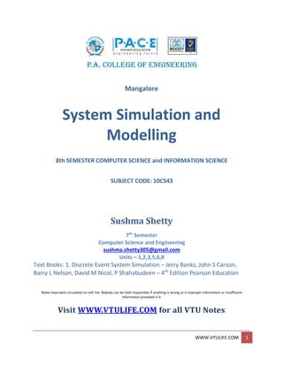
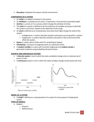
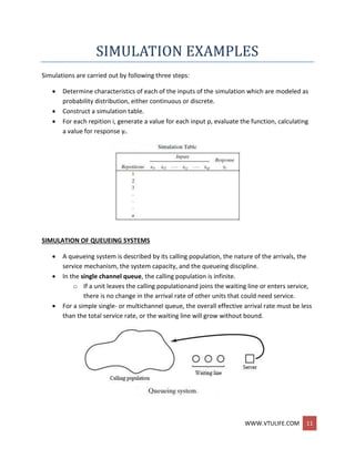
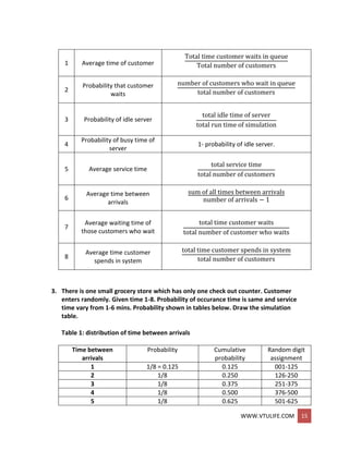
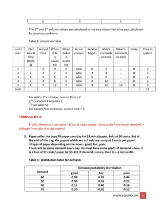
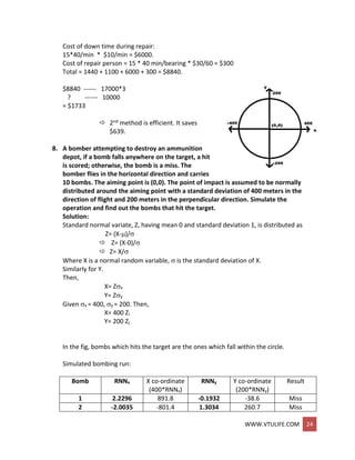
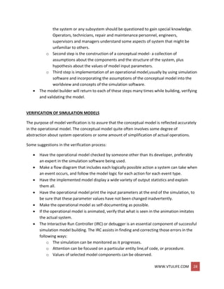
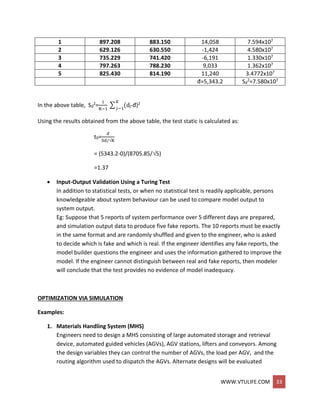
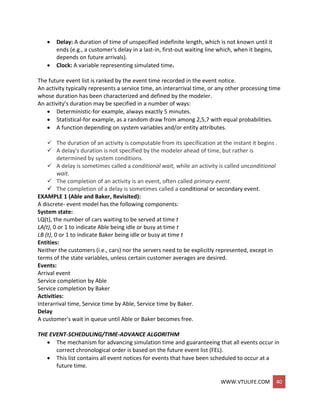
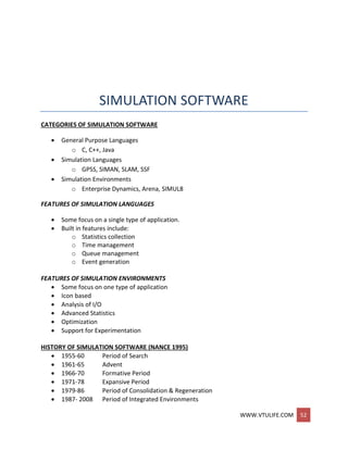
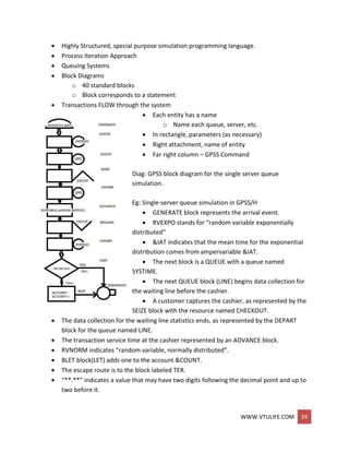
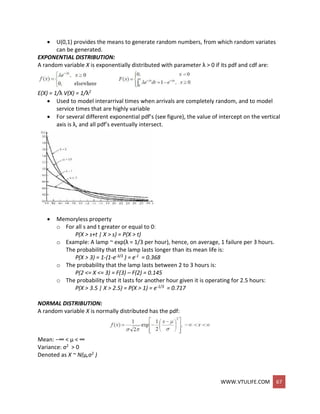
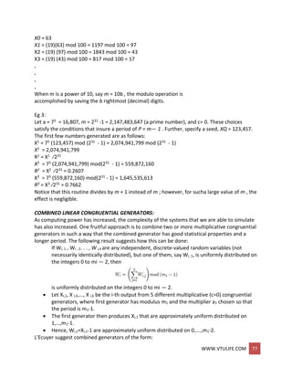
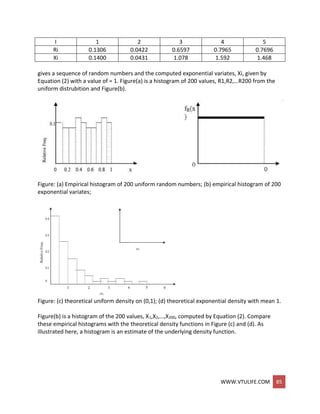
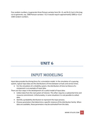
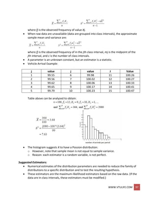
Table 3: bearing replacement under current methods.
Bearing 1 Bearing 2 Bearing 3
RDa life RD delay RDb life RD delay RDc life RD delay
67 1400 7 10 71 1500 8 10 18 1100 6 5
57 1300 3 5 21 1100 3 5 17 1100 2 5
98 1900 1 5 79 1500 3 5 65 1400 2 5
76 1500 6 5 88 1700 1 5 3 1000 9 10
53 1300 4 5 93 1800 0 15 54 1300 8 10
69 1400 8 10 77 1500 6 5 17 1100 3 5
80 1500 5 5 8 1000 9 10 19 1100 6 5
93 1800 7 5 21 1100 8 10 9 1000 7 10
35 1200 0 10 13 1100 3 5 61 1300 1 5
02 1000 5 5 3 1000 2 5 84 1600 0 15
99 1900 9 10 14 1100 1 5 11 1100 5 5
65 1400 4 5 5 1000 0 15 25 1200 2 5
53 1300 7 10 29 1200 2 5 86 1700 8 10
87 1700 1 5 7 1000 4 5 65 1400 3 5
90 1700 2 5 20 1100 3 5 44 1200 4 5
total 22300 110 18700 110 18600 105
Number of bearings= 3 (bearings) * 15 (tuples) = 45.
Cost of bearings:
45 bearings * $32 / bearing = $1440
Cost of delay:
(110+110+105) * $10 / min = $3250
Cost of down time during repairs:
45 bearings * 20 min/ bearing * $30/60 min = $9000
Cost of repair person:
45 bearings * 20 min/ bearing * $30 / 60 min = $450
Total cost = $1440+ $3250+ $9000+ $450 = $14140
Total bearing 1+bearing 2+bearing 3 [life] = 22300+18700+18600 =
59600 hrs.
Total cost = $23720 // cross multiplication of
$14140 ---- 59600 hrs
? ---- 10000 hrs
New proposal:
Total bearing hours = 17000.
Delay to change = 110 hrs.
45 bearing * $32/bearing = $1440
Cost of delay = 110 * $10/min = $1100
45/3=15.

24. WWW.VTULIFE.COM 24
Cost of down time during repair:
15*40/min * $10/min = $6000.
Cost of repair person = 15 * 40 min/bearing * $30/60 = $300
Total = 1440 + 1100 + 6000 + 300 = $8840.
$8840 ------ 17000*3
? ------ 10000
= $1733
 2nd method is efficient. It saves
$639.
8. A bomber attempting to destroy an ammunition
depot, if a bomb falls anywhere on the target, a hit
is scored; otherwise, the bomb is a miss. The
bomber flies in the horizontal direction and carries
10 bombs. The aiming point is (0,0). The point of impact is assumed to be normally
distributed around the aiming point with a standard deviation of 400 meters in the
direction of flight and 200 meters in the perpendicular direction. Simulate the
operation and find out the bombs that hit the target.
Solution:
Standard normal variate, Z, having mean 0 and standard deviation 1, is distributed as
Z= (X-)/
 Z= (X-0)/
 Z= X/
Where X is a normal random variable,  is the standard deviation of X.
Similarly for Y.
Then,
X= Zx
Y= Zy
Given x = 400, y = 200. Then,
X= 400 Zi
Y= 200 Zj
In the fig, bombs which hits the target are the ones which fall within the circle.
Simulated bombing run:
Bomb RNNx X co-ordinate
(400*RNNx)
RNNy Y co-ordinate
(200*RNNy)
Result
1 2.2296 891.8 -0.1932 -38.6 Miss
2 -2.0035 -801.4 1.3034 260.7 Miss

25. WWW.VTULIFE.COM 25
3 -3.1432 -1257.3 0.3286 65.7 Miss
4 -0.7968 -318.7 -1.1417 -228.3 Miss
5 1.0741 429.6 0.7612 152.2 Hit
6 0.1265 50.6 -0.3098 -62.0 Hit
7 0.0611 24.5 -1.1066 -221.3 Hit
8 1.2182 487.3 0.2487 49.7 Hit
9 -0.8026 -321.0 -1.0098 -202.0 Miss
10 0.7324 293.0 0.2552 -51.0 Hit
9. Suppose the max inventory level M is 10 units. Review period is 3 days. Estimate by
simulation the average ending units in inventory and number of days when a shortage
occurs. The number of units demanded/day is given by the following demand
distribution table.
Assume that orders are placed at the end of the business and are received at the
beginning of business determined by the lead time. Initially simulation has started
with inventory level of 3 units and an order of 5 units scheduled to arrive in 2 days
time.
Table 1: demand distribution table
demand probability Cumulative
probability
Random digit
0 0.10 0.10 01-10
1 0.25 0.35 11-35
2 0.35 0.70 36-70
3 0.21 0.91 71-91
4 0.09 1.00 92-00
Table 2: lead time distribution
Lead time Probability Cumulative
probability
Random digit
1 0.6 0.6 1-6
2 0.3 0.9 7-9
3 0.1 1.0 0-0
Random digits for demand: 24, 65, 35, 81, 52, 3, 27, 73, 70, 47, 45, 48, 17, 9, 87.
Random digit for lead time: 5,1,3,5,1.
Solution: ( similar to prob number 6)
Table 3: Simulation table

26. WWW.VTULIFE.COM 26
Day cycle Begin
inventory
RD for
demand
demand End of
inventory
shortage Order
quantity
RD
for
lead
time
Days left
for order
to arrive
1 1 3 24 1 2 - - - 1
2 1 2 65 2 0 - - - 0
3 1 0+5=5 35 1 4 - 6 5 1
1 2 4 81 3 1 - - - 0
2 2 1+6=7 52 2 5 - - - -
3 2 5 3 0 5 - 5 1 1
1 3 5 27 1 4 - - - 0
2 3 4+5=9 73 3 6 - - - -
3 3 6 70 2 4 - 6 3 1
1 4 4 47 2 2 - - - 0
2 4 2+6=8 45 2 6 - - - -
3 4 6 48 2 4 - 6 5 1
1 5 4 17 1 3 - - - 0
2 5 3+6=9 9 0 9 - - - -
3 5 9 87 3 6 - 4 1 1

27. WWW.VTULIFE.COM 27
UNIT 8
VERIFICATION AND VALIDATION OF
SIMULATION MODELS
VERIFICATION: is concerned with building the model correctly. It proceedes by comparison of
the conceptual model to the comuter representation that implements that conception.
VALIDATION: is concerned with building the correct model. It attempts to confirm that a model
is an accurate representation of the real system. It is achieved through the caliberation of the
model.
GOAL OF THE VALIDATION PROCESS:
 To produce a model that represents true system behaviour closely enough for the
model to be used as a substitute for the actual
system for the purpose of experimenting with the
system, analyzing system behaviour and predicting
system performance.
 To increase to an acceptable level the credibility of
the model, so that the model will be used by
managers and other decision makers.
MODEL BUILDING, VERIFICATION AND VALIDATION
 Model building:
o First step consists of observing the real
system and the interaction among their
various components and of collecting data
on their behaviour. Persons familiar with

28. WWW.VTULIFE.COM 28
the system or any subsystem should be questioned to gain special knowledge.
Operators, technicians, repair and maintenance personnel, engineers,
supervisors and managers understand some aspects of system that might be
unfamiliar to others.
o Second step is the construction of a conceptual model- a collection of
assumptions about the components and the structure of the system, plus
hypothesis about the values of model input parameters.
o Third step is implementation of an operational model,usually by using simulation
software and incorporating the assumptions of the conceptual model into the
worldview and concepts of the simulation software.
 The model builder will return to each of these steps many times while building, verifying
and validating the model.
VERIFICATION OF SIMULATION MODELS
The purpose of model verification is to assure that the conceptual model is reflected accurately
in the operational model. The conceptual model quite often involves some degree of
abstraction about system operations or some amount of simplification of actual operations.
Some suggestions in the verification process:
 Have the operational model checked by someone other than its developer, preferably
an expert in the simulation software being used.
 Make a flow diagram that includes each logically possible action a system can take when
an event occurs, and follow the model logic for each action for each event type.
 Have the implemented model display a wide variety of output statistics and explain
them all.
 Have the operational model print the input parameters at the end of the simulation, to
be sure that these parameter values have not been changed inadvertently.
 Make the operational model as self-documenting as possible.
 If the operational model is animated, verify that what is seen in the animation imitates
the actual system.
 The Interactive Run Controller (IRC) or debugger is an essential component of successful
simulation model building. The IRC assists in finding and correcting those errors in the
following ways:
o The simulation can be monitored as it progresses.
o Attention can be focused on a particular entity line,of code, or procedure.
o Values of selected model components can be observed.

29. WWW.VTULIFE.COM 29
o The simulation can be temporarily suspended, or paused, not only to view
information, but also to reassign values or redirect entities.
 Graphical interfaces are
recommended for accomplishing
verification and validation.
PROBLEM 1:
When verifying the operational model (in
a general purpose language such as FORTRAN, Pascal, C or C++, or most simulation languages)
of the single-server queue model asin fig below:
An analyst made a run over 16 units of time and observed that the time-coverage length of the
waiting line was LQ customer.
The table below gives the hypothetical printout from simulation time CLOCK=0 to CLOCK=16 for
the simple single server queue (fig above).
Definition of variables:
CLOCK = simulation clock
EVTYP = event type (start,arrival,departure or stop)
NCUST = number of customers in system at time ‘CLOCK’
STATUS = status of server (1-busy, 0-idle)
State of system just after the named event occurs:
CLOCK=0 EVTYP=’start’ NCUST=0 STATUS=0
CLOCK=3 EVTYP=’arrival’ NCUST=1 STATUS=0
CLOCK=5 EVTYP=’depart’ NCUST=0 STATUS=0
CLOCK=11 EVTYP=’arrival’ NCUST=1 STATUS=0
CLOCK=12 EVTYP=’arrival’ NCUST=2 STATUS=1
CLOCK=16 EVTYP=’depart’ NCUST=1 STATUS=1
The LQ is calculated as:
// (NCUSTi-STATUSi)*(CLOCKi+1-CLOCKi)
LQ =
(0−0)∗(3−0) + (1−0)∗(5−3)+ (0−0)∗(11−5)+ (1−0)∗(12−11)+ (2−1)∗(16−12)
(3−0)+(5−3)+(11−5)+(12−11)+(16−12)
= 7/16 = 0.4375
CALIBERATION AND VALIDATION OF MODELS

30. WWW.VTULIFE.COM 30
 Verification and validation, although conceptually distinct, usually are conducted
simultaneously by the modeler.
 Validation is the overall process of
comparing the model and its behaviour to
the real system and its behaviour.
 Caliberation is the iterative process of
comparing the model to the real system,
making additional adjustments (or even
major changes) to the model, comparing the
revised model to reality, making additional
adjustments, comparing again, and so on.
 Fig below shows the relationship of model
caliberation to the overall validation process.
 The comparison of the model to reality is
carried out by a variety of tests – some
subjective and others objective.
o Subjective : usually involve people, who are knowledgeable about one or mode
aspects of the system, making judgements about the model and its output.
o Objective : require data on the system’s behaviour, also corresponding data
produced by the model.
o Then one or more statistical tests are performed to compare some aspect of the
system data set with the same aspect of the model data set.
 This iterative process of comparing model with system and then revising both the
conceptual and operational models to accommodate any perceived model deficiencies
is continued until the model is judged to be sufficiently accurate.
 Naylor and Finger formulated a three-step approach that has been widely followed.
o Build a model that has high face validity.
o Validate model assumptions
o Compare the model input-output transformations to corresponding input-output
transformations for the real system.
 Face validity:
o The first goal of the simulation modeler is to construct a model that appears
reasonable on its face to model users and others who are knowledgeable about
the real system being simulated.
o Potential users and knowledgeable persons can also evaluate model output for
reasonableness and can aid in identifying model deficiencies.

31. WWW.VTULIFE.COM 31
o Sensitivity analysis can also be used to check a model’s face validity. The model
user is asked whether the model behaves in the expected way when one or more
input variables are changed.
 Validation of model assumptions:
o Model assumptions fall into two general classes:
 Structural assumptions: involve questions of how the system operates
and usually involve simplifications and abstractions of reality.
 Data assumptions: should be based on the collection of reliable data and
correct statistical analysis of the data.
o The use of goodness-of-fit tests is an important part of the validation of data
assumptions.
 Validating input-output transformations:
o The ultimate test of a model, and in fact the only objective test of the model as a
whole, is the model’s ability to predict the future behaviour of the real system
when the model input data match the real inputs and when a policy
implemented at some point in the system.
o The structure of the model must be accurate enough for the model to make
good predictions, not just for one input data set, but for the range of input data
sets that are of interest.
o The modeler can also use historical data that have been reserved for validation
purposes only.
o In any case, the modeler should use the main responses of interest as the
primary criteria for validating a model.
o The model will be used to compare alternative system designs or to investigate
system behaviour under a range of new input conditions.
o First, the responses of the two models under similar input conditions will be
used as the criteria for comparison of the existing system to the proposed
system.
o Second, in many cases the proposed system is a modification of the existing
system and the modeler hopes that confidence in the model of the existing
system can be transferred to the model of the new system.
 Input-output validation: Using historical input data:
o When using artificially generated data as input data, the modeler expects the
model to produce event patterns that are compatible with but not identical to,
that event patterns that occurred in the real system during the period of data
collection.
o An alternative to generating input data is to use the actual historical record, to
drive the simulation model and then to compare model output with system data.

32. WWW.VTULIFE.COM 32
o Event scheduling without random number generation could be implemented
quiet easily in a general purpose programming language or most simulation
languages by using arrays to store the data or reading the data from the file.
o When using the above technique, the modeler hopes that the simulation will
duplicate as closely as possible the important events that occurred in the real
system.
o In some systems, electronic counters and devices are used to ease the data
collection task by automatically recording certain types of data.
 Input-output validation: Using a turing test:
o In addition to statistical tests, or when no statistical test is readily applicable,
persons knowledgeable about system behaviour can be used to compare model
output to system output.
o System performance reports are randomly shuffled and given to the engineer,
who is asked to decide which reports are fake and which are real.
o If the engineer cannot distinguish between fake and real reports with any
consistency, the modeler will conclude that the
test provides no evidence of model inadequacy.
PROBLEM 2:
The production line at the Sweet Lil’ Things Candy Factory in
Decatur consists of three machines that make package, and
box their famous candy. One machine (the candy maker)
makes and wraps individual pieces of candy and sends them
by conveyor to the packer. The second machine (the packer)
packs the individual pieces into a box. A third machine (the
box maker) forms the boxes and supplies them by conveyor to
the packer. The system is illustrated as in fig.
Validation of the Candy-Factory Model:
Response, i System, Zi Model, Yi
1. Production level 897.208 883,150
2. Number of operator
interventions
3 3
3. Time of occurance 7:22, 8:41, 10:10 7:24, 8:42, 10:14
Input data set j System
production,
Zij
Model
production, Wij
Observed
difference,
dj=Zij-Wij
Squared
Deviation from
Mean, (dj-đ)2

33. WWW.VTULIFE.COM 33
1 897.208 883.150 14,058 7.594x107
2 629.126 630.550 -1,424 4.580x107
3 735.229 741.420 -6,191 1.330x107
4 797.263 788.230 9,033 1.362x107
5 825.430 814.190 11,240 3.4772x107
đ=5,343.2 Sd
2=7.580x107
In the above table, Sd
2=
1
K−1
∑ (d
𝐾
𝑗−1
j-đ)2
Using the results obtained from the above table, the test static is calculated as:
t0=
đ
Sd/K
= (5343.2-0)/(8705.85/5)
=1.37
 Input-Output Validation Using a Turing Test
In addition to statistical tests, or when no statistical test is readily applicable, persons
knowledgeable about system behaviour can be used to compare model output to
system output.
Eg: Suppose that 5 reports of system performance over 5 different days are prepared,
and simulation output data to produce five fake reports. The 10 reports must be exactly
in the same format and are randomly shuffled and given to the engineer, who is asked
to decide which is fake and which is real. If the engineer identifies any fake reports, the
model builder questions the engineer and uses the information gathered to improve the
model. If the engineer cannot distinguish between real and fake reports, then modeler
will conclude that the test provides no evidence of model inadequacy.
OPTIMIZATION VIA SIMULATION
Examples:
1. Materials Handling System (MHS)
Engineers need to design a MHS consisting of large automated storage and retrieval
device, automated guided vehicles (AGVs), AGV stations, lifters and conveyors. Among
the design variables they can control the number of AGVs, the load per AGV, and the
routing algorithm used to dispatch the AGVs. Alternate designs will be evaluated

34. WWW.VTULIFE.COM 34
according to AGV utilization, transportation delay for material that needs to be moved,
and overall investment and operation costs.
2. Liquified Natural Gas (LNG) Transportation
A LNG transportation system will consist of Lng tankers and of loading, unloading and
storage facilities in order to minimize cost, designers can control tanker size, number of
tankers in use, capacity of storage tanks.
3. Automobile Engine Assembly
In an assembly line, a large buffer between workstations could increase station
utilization. An allocation of buffer capacity that minimizes the sum of these competing
costs is desired.
4. Traffic Signal Sequencing
Civil engineers want to sequence the traffic signals along the busy section of road to
reduce driver delay and the conjestion occurring along narrow cross streets. For each
traffic signal the length of the red, green and green-turn-arrow cycle can be set
individually.
5. On-line services
A company offering on-line information services over the internet is changing its
computer architecture from central mainframe computers to distributed workstation
computing. The numbers and types of CPUs, the network structure and the allocation of
processing tasks all need to be chosen. Response time to customer queries is the key
performance measure.
All of these problems fall under the general topic of “optimization via simulation”,
where the goal is to minimize or maximize some measures some measures of system
performance and system performance can be evaluated only by running a computer
simulation.
OPTIMIZATION VIA SIMULATION
 Optimization is a key tool used by operations researchers and management scientists
and there are well developed algorithms for many classes of problems , the most
famous being linear programming.
 Much of the work on optimization deals with problems in which all aspects of the
system are treated as being known with certainity; most critically, the performance of
any design (cost, profit, makespan etc) can be evaluated exactly.
 In stochastic, discrete event simulation, the result of any simulation run is a random
variable. For notation, let x1,x2,….,xm be the m controllable design variables and let
Y(x1,x2,….,xm) be the observed simulation output performance on the run. To be
concrete x1,x2,x3 might denote member of AGVs, the load per AGV, and the routing
algorithm used to dispatch the AGVs respectively.

35. WWW.VTULIFE.COM 35
 To optimize Y(x1,x2,….,xm) with respect to x1,x2,….,xm
o Maximize or minimize E(Y(x1,x2,….,xm)).
The mathematical expectation or long run average.
 For instance we might want to select the MHS design that has the best chance of costing
less than SD to purchase and operate changing the objective to
Maximize Pr(Y(x1,x2,….,xm)<=D)
We can fit this objective into formulation by defining a new performace measure
Y(x1,x2,….,xm) = {
𝑖, 𝑖𝑓 Y(x1, x2, … . , xm) ≤ 0
0, otherwise
and maximizing E(Y(x1,x2,….,xm)) instead.
 At present, multiple objective optimization via simulation is not well developed. Thus,
one of the three strategies is developed.
o Combine all of the performance measures into a single measure, the most
common being cost.
o Optimize with respect to one key performance measure, but then evaluate the
top solutions with respect to secondary performance measures.
o Optimize with respect to one key performance measure, but consider only those
alternatives that meet certain constraints on the other performance measures.
WHY IS OPTIMIZATION VIA SIMULATION DIFFICULT?
 Even when there is no uncertainity,noptimization can be very difficult if the number of
design variables is large.
 Optimization via simulation adds an additional complication: The performance of a
particular design cannot be evaluated exactly, but instead must be estimated.
 The existence of sampling variability forces optimization via simulation to make
compromises. The following are standard ones:
o Generate a prespecified probability of correct selection:
Eg: The two stage Bonferroni procedure. This allows the analyst to specify the
desired chance of being right.
o Guarantee asymptotic convergence: There are many algorithms that guarantee
convergence to the global optimal solution as the simulation effort becomes
infinite. These guarantees are useful because they indicate that the algorithm
tends to get to where the analyst wants it to go.

36. WWW.VTULIFE.COM 36
o Optimal for deterministic counterpart: The idea here is to use an algorithm that
would find the optimal solution if the performance of each design could be
evaluated with certainity.
o Robust heuristics: many heuristics have been developed for deterministic
optimization problems that do not guarantee finding the optimal solutions, but
nevertheless been shown to be very effective on difficult, practical problems.
USING ROBUST HEURISTICS
 The procedure does not depend on strong problem structure- such as continuity or
convexity of E(Y(x1,x2,…..,xm)), to be effective, can be applied to problems with mixed
type of decision variables and is tolerant to some sampling variability. Eg: Generic
algorithms(GA) and tabu search (TS).
 Algorithm:
BASIC GA
step 1: Set the iteration counter j=0, and select an initial population of p solutions
P(0)={x1(0),…..,xp(0)}
step 2: Run simulation experiments to obtain performance estimates Y(x) for all p
solutions x(j) in P(j).
step 3: Select a population of p solutions from those in P(j) in such a way that those with
smaller Y(x) values are more likely, but not certain, to be selected. Denote this
population of solutions as P(j+1).
step 4: Recombine the solutions in P(j+1) via crossover (which joins parts of two
solutions xt(j+1) and xl(j+1) to form new solution) and mutation (which randomly
changes a part of solution xi(j+1).
step 5: Set j=j+1 and goto step 2.
The GA can be terminated after a specified number of iterations, when little or no
improvement is noted in the population, or when the population contains p copies of
the same solution. At termination, the solution x* that has the smallest Y(x) value in the
last population is chosen as the best.
BASIC TS
Step 1: set the iteration counter j=0 and the list of tabu moves to empty. Select an initial
solution x* in X.
Step 2: find the solution x that minimizes Y(x) over all of the neighbours of x* that are
not received by tabu moves, running whatever simulation are needed to do the
optimization.
Step 3: if Y(xy)<Y(x*) , then x*…y

37. WWW.VTULIFE.COM 37
Step 4: update the list of tabu moves and go to step 2.
The TS can be terminated when a specified number of iterations have been completed,
when some number of iterations has passed without changing x*, or when there are no
feasible moves. At termination the solution x* is chosen as best.
 Control sampling variability:
o In many cases, it will be upto the user to determine how much sampling will be
undertaken at each potential solution. This is a difficult problem in general.
o If the analyst must specify a fixed number of replications per solution that will be
used through the search, then a preliminary experiment must be conducted.
o Simulate several designs, some at the extremes of the solution space and some
nearer the center. Compare the apparent best and apparent worst of these
designs.
o Find the minimum for the number of replications required to declare these
designs to be statistically significantly different.
o After optimization run has been completed, perform a second set of experiments
on the top 5 to 10 designs identified by the heuristic. Use the comparison
techniques to rigorously evaluate which are the best or near-best of these
designs.
 Restarting:
o If people familiar with the system suspect that certain designs will be good, be
sure to module them as possible starting solutions for the heuristic.
RANDOM SEARCH
 Let the k possible solutions to the optimization via simulation problem be denoted
{xi1,xi2,….,xim} provides specific settings for the m decision variables. The simulation
output at xi is denoted Y(xi) ; this could be the output of a single replication or the
average of several replications. We need to find x* that minimizes E(Y(x)).
 Algorithm:
Step 1: Initialize counter variables C(i)=0 for i=1,2,….k. Select an initial solution i0, and
set C(i0)=1.
Step 2: Choose another solution i’ from the set of all solutions except i0 in such a way
that each solution has an equal chance of being selected.
Step 3: Run simulation experiments at the two solutions i0 and i’ to obtain outputs Y(i0)
and Y(i’). if Y(i’)<Y(i0), then set i0=i’.
Step 4: Set C(i0)=C(i0)+1. If not done, then goto step 2. If done, then select as the
estimated optimal solution xi* such that C(i*) is the largest count.

38. WWW.VTULIFE.COM 38
If there is a maximization problem, replace step 3 with
Step 3: Run simulation experiments at the two solutions i0 and i’ to obtain outputs Y(i0)
and Y(i’). if Y(i’)>Y(i0), then set i0=i’.

39. WWW.VTULIFE.COM 39
UNIT 2
GENERAL PRINCIPLES
In discrete-event simulation, a system is modeled in terms of its state at each point in time; the
entities that pass through the system and the entities that rep-j resent system resources; and
the activities and events that cause system state to change.
CONCEPTS IN DISCRETE-EVENT SIMULATION
To develop a framework for the development of a discrete-event model of a system. The major
concepts are briefly defined and then illustrated
with examples:
 System: A collection of entities (e.g., people and machines) that ii together over time to
accomplish one or more goals.
 Model: An abstract representation of a system, usually containing structural, logical, or
mathematical relationships which describe a system in terms of state, entities and their
attributes, sets, processes, events, activities, and delays.
 System state: A collection of variables that contain all the information necessary to
describe the system at any time.
 Entity: Any object or component in the system which requires explicit representation in
the model (e.g., a server, a customer, a machine).
 Attributes: The properties of a given entity (e.g., the priority of a v customer, the
routing of a job through a job shop).
 List: A collection of (permanently or temporarily) associated entities ordered in some
logical fashion (such as all customers currently in a waiting line, ordered by first come,
first served, or by priority).
 Event: An instantaneous occurrence that changes the state of a system as an arrival of a
new customer).
 Event notice: A record of an event to occur at the current or some future time, along
with any associated data necessary to execute the event; at a minimum, the record
includes the event type and the event time.
 Event list: A list of event notices for future events, ordered by time of occurrence; also
known as the future event list (FEL).
 Activity: A duration of time of specified length (e.g., a service time or arrival time),
which is known when it begins (although it may be defined in terms of a statistical
distribution).

40. WWW.VTULIFE.COM 40
 Delay: A duration of time of unspecified indefinite length, which is not known until it
ends (e.g., a customer's delay in a last-in, first-out waiting line which, when it begins,
depends on future arrivals).
 Clock: A variable representing simulated time.
The future event list is ranked by the event time recorded in the event notice.
An activity typically represents a service time, an interarrival time, or any other processing time
whose duration has been characterized and defined by the modeler.
An activity’s duration may be specified in a number of ways:
 Deterministic-for example, always exactly 5 minutes.
 Statistical-for example, as a random draw from among 2,5,7 with equal probabilities.
 A function depending on system variables and/or entity attributes.
 The duration of an activity is computable from its specification at the instant it begins .
 A delay's duration is not specified by the modeler ahead of time, but rather is
determined by system conditions.
 A delay is sometimes called a conditional wait, while an activity is called unconditional
wait.
 The completion of an activity is an event, often called primary event.
 The completion of a delay is sometimes called a conditional or secondary event.
EXAMPLE 1 (Able and Baker, Revisited):
A discrete- event model has the following components:
System state:
LQ(t), the number of cars waiting to be served at time t
LA(t), 0 or 1 to indicate Able being idle or busy at time t
LB (t), 0 or 1 to indicate Baker being idle or busy at time t
Entities:
Neither the customers (i.e., cars) nor the servers need to be explicitly represented, except in
terms of the state variables, unless certain customer averages are desired.
Events:
Arrival event
Service completion by Able
Service completion by Baker
Activities:
Interarrival time, Service time by Able, Service time by Baker.
Delay
A customer's wait in queue until Able or Baker becomes free.
THE EVENT-SCHEDULING/TIME-ADVANCE ALGORITHM
 The mechanism for advancing simulation time and guaranteeing that all events occur in
correct chronological order is based on the future event list (FEL).
 This list contains all event notices for events that have been scheduled to occur at a
future time.

41. WWW.VTULIFE.COM 41
 At any given time t, the FEL contains all previously scheduled future events and their
associated event times.
 The FEL is ordered by event time, meaning that the events are arranged chronologically;
that is, the event times satisfy
t < t1 <= t2 <= t3 <= ….,<= tn
t is the value of CLOCK, the current value of simulated time. The event dated with time
t1 is called the imminent event; that is, it is the next event will occur. After the system
snapshot at simulation time CLOCK == t has been updated, the CLOCK is advanced to
simulation time CLOCK _= t1 and the imminent event notice is removed from the FEL
and the event executed.. This process repeats until the simulation is over.
 The sequence of actions which a simulator must perform to advance the clock system
snapshot is called the event-scheduling/time-advance algorithm.
Old system snapshot at time t
Event-scheduling/time-advance algorithm:
Step 1. Remove the event notice for the imminent event (event 3, time t) from PEL
Step 2. Advance CLOCK to imminent event time (i.e., advance CLOCK from r to t1).
Step 3. Execute imminent event: update system state, change entity attributes, and set
membership as needed.
Step 4. Generate future events (if necessary) and place their event notices on PEL ranked by
event time. (Example: Event 4 to occur at time t*, where t2 < t* < t3.)
Step 5. Update cumulative statistics and counters.
New system snapshot at time t1

42. WWW.VTULIFE.COM 42
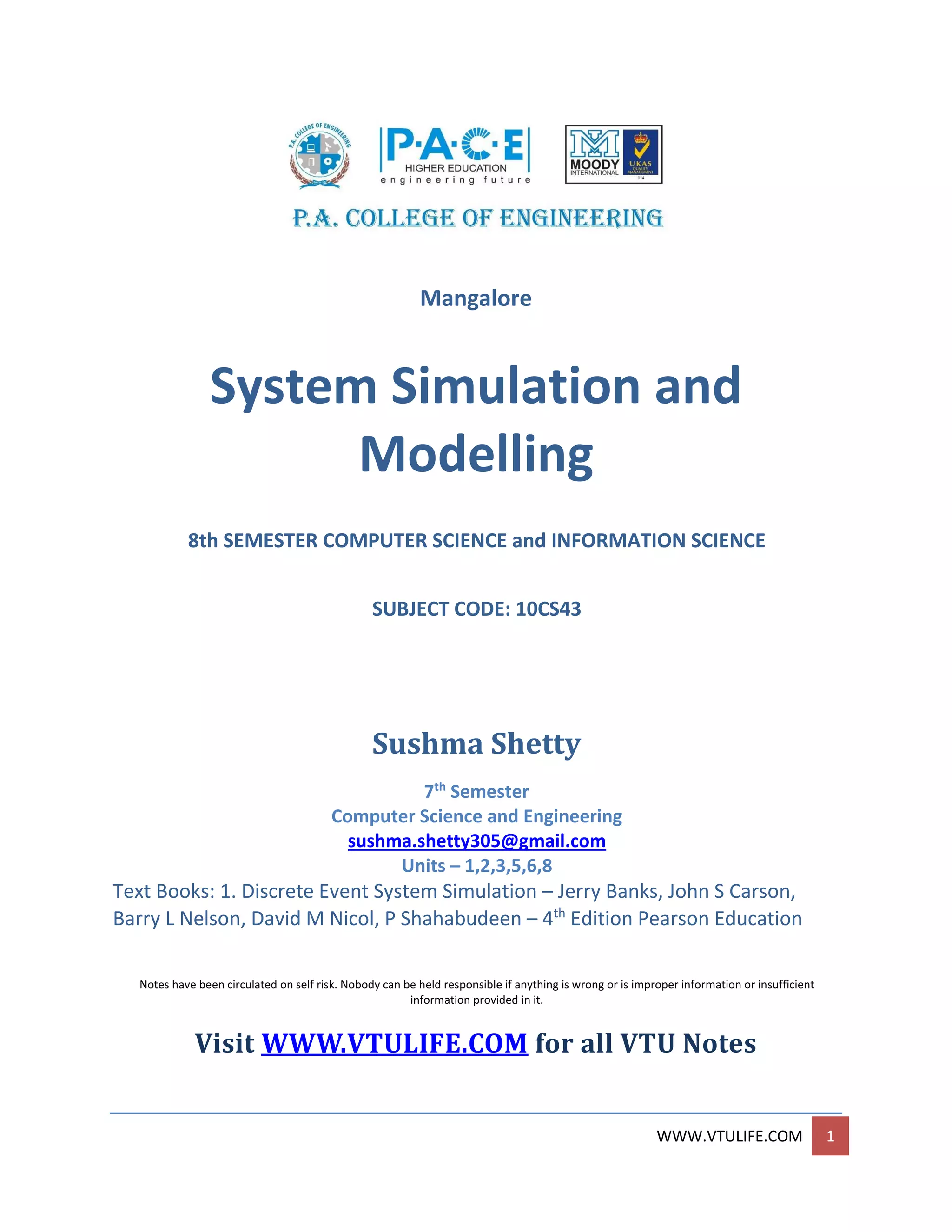
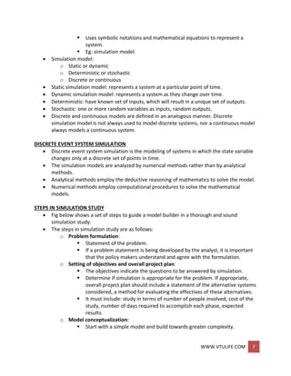
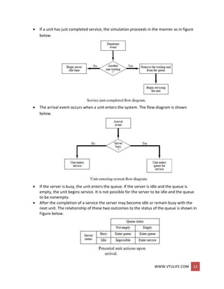
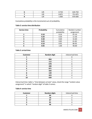
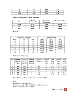
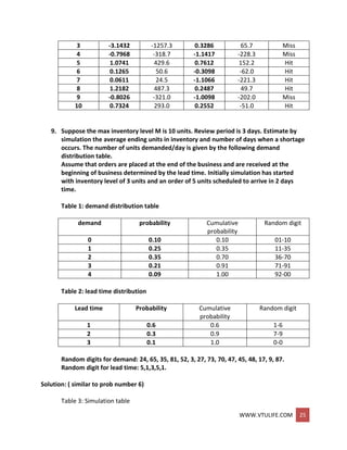
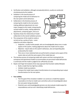
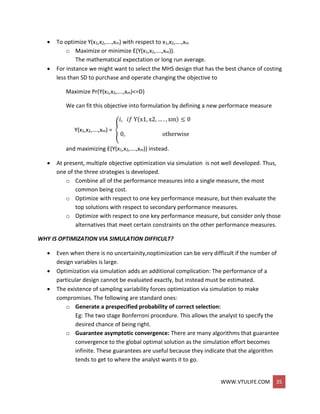
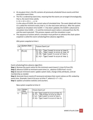
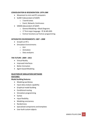
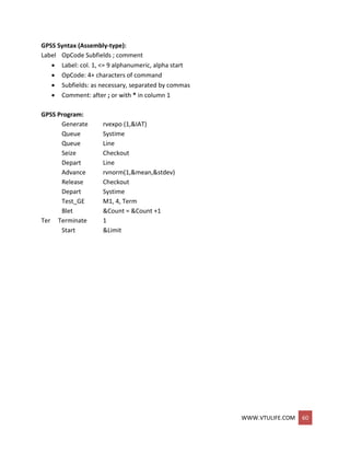
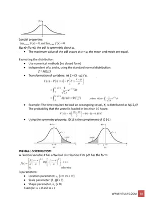
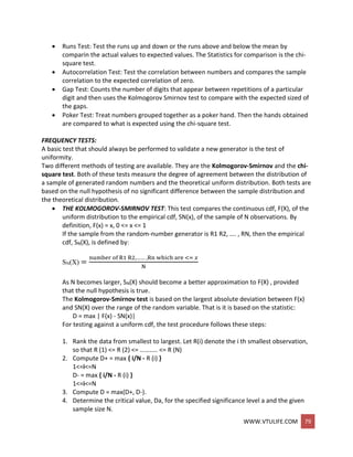
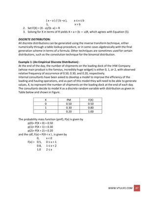
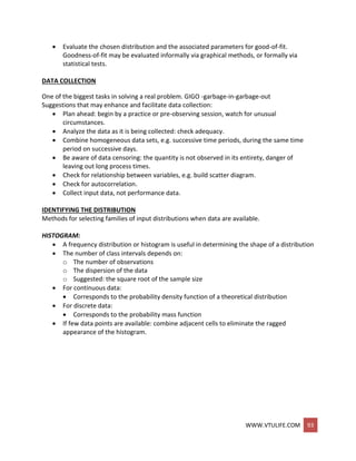
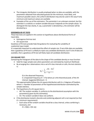
Advancing simulation time and updating system image
 The management of a list is called list processing.
 The major list processing operations performed on a FEL are removal of the imminent
event, addition of a new event to the list, and occasionally removal of some event
(called cancellation of an event).
 As the imminent event is usually at the top of the list, its removal is as efficient as
possible. Addition of a new event (and cancellation of an old event) requires a search of
the list.
 The removal and addition of events from the PEL is illustrated in figure above.
o When event 4 (say, an arrival event) with event time t* is generated at step 4,
one possible way to determine its correct position on the FEL is to conduct a top-
down search:
If t* < t2, place event 4 at the top of the FEL.
If t2 < t* < t3, place event 4 second on the list.
If t3, < t* < t4, place event 4 third on the list.
If tn < t*, event 4 last on the list.
o Another way is to conduct a bottom-up search.
 The system snapshot at time 0 is defined by the initial conditions and the generation of
the so-called exogenous events.
 The method of generating an external arrival stream, called bootstrapping.
 Every simulation must have a stopping event, here called E, which defines how long the
simulation will run. There are generally two ways to stop a simulation:
o At time 0, schedule a stop simulation event at a specified future time TE. Thus,
before simulating, it is known that the simulation will run over the time interval
[0, TE].
Example: Simulate a job shop for TE = 40 hours.
o Run length TE is determined by the simulation itself. Generally, TE is the time of
occurrence of some specified event E.
Examples: TE is the time of the 100th service completion at a certain service
center. TE is the time of breakdown of a complex system.
WORLD VIEWS
 When using a simulation package or even when using a manual simulation, a modeler
adopts a world view or orientation for developing a model.
 Those most prevalent are the event scheduling world view, the process-interaction
worldview, and the activity-scanning world view.
 When using a package that supports the process-interaction approach, a simulation
analyst thinks in terms of processes .
 When using the event-scheduling approach, a simulation analyst concentrates on events
and their effect on system state.

43. WWW.VTULIFE.COM 43
 The process-interaction approach is popular because of its intuitive appeal, and because
the simulation packages that implement it allow an analyst to describe the process flow
in terms of high-level block or network constructs.
 Both the event-scheduling and the process-interaction approaches use a / variable time
advance.
 The activity-scanning approach uses a fixed time increment and a rule-based approach
to decide whether any activities can begin at each point in simulated time.
 The pure activity scanning approach has been modified by what is called the three-
phase approach.
 In the three-phase approach, events are considered to be activity duration-zero time
units. With this definition, activities are divided into two categories called B and C.
o B activities: Activities bound to occur; all primary events and unconditional
activities.
o C activities: Activities or events that are conditional upon certain conditions
being true.
 With the. three-phase approach the simulation proceeds with repeated execution of the
three phases until it is completed:
o Phase A: Remove the imminent event from the FEL and advance the clock to its
event time. Remove any other events from the FEL that have the event time.
o Phase B: Execute all B-type events that were removed from the FEL.
o Phase C: Scan the conditions that trigger each C-type activity and activate any
whose conditions are met. Rescan until no additional C-type activities can begin
or events occur.
 The three-phase approach improves the execution efficiency of the activity scanning
method.
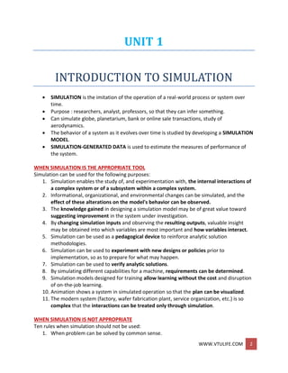
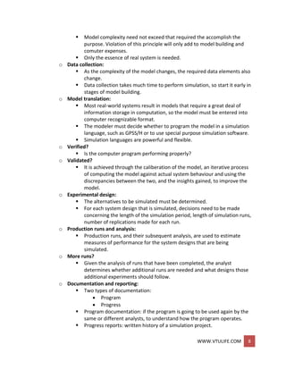
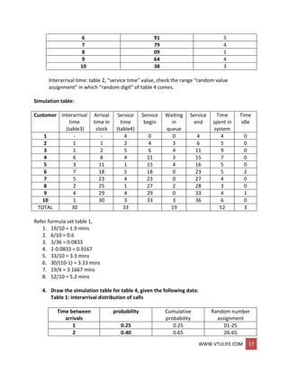
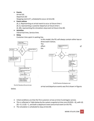
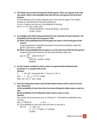
EXAMPLE: (Able and Baker, Back Again)
Using the three-phase approach, the conditions for beginning each activity in Phase C are:
Activity Condition
Service time by Able: A customer is in queue and Able is idle,
Service time by Baker: A customer is in queue, Baker is idle, and Able is busy.
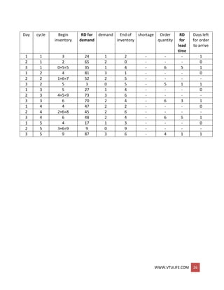
MANUAL SIMULATION USING EVENT SCHEDULING
In an event-scheduling simulation, a simulation table is used to record the successive system
snapshots as time advances. Lets consider the example of a grocery shop which has only one
checkout counter.
Example: (Single-Channel Queue)
The system consists of those customers in the waiting line plus the one (if any) checking out.
The model has the following components:
System state (LQ(i), Z,S(r)), where LQ((] is the number of customers in the waiting line, and LS(t)
is the number being served (0 or 1) at time t.
 Entities The server and customers are not explicitly modeled, except in terms of the
state variables above.

44. WWW.VTULIFE.COM 44
 Events
Arrival (A)
Departure (D)
Stopping event (£"), scheduled to occur at time 60.
 Event notices
(A, i). Representing an arrival event to occur at future time t.
(D, t), representing a customer departure at future time t.
(£, 60), representing the simulation-stop event at future time 60.
 Activities
Inlerarrival time, Service time.
 Delay
Customer time spent in waiting line.
In this model, the FEL will always contain either two or
three event notices.
The
effect of
the
arrival and departure events was first shown in Figures
below.
 Initial conditions are that the first customer arrives at time 0 and begins service.
 This is reflected in Table below by the system snapshot at time zero (CLOCK = 0), with LQ
(0) = 0, LS (0) = 1, and both a departure event and arrival event on the FEL.
 The simulation is scheduled to stop at time 60.

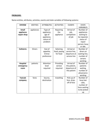
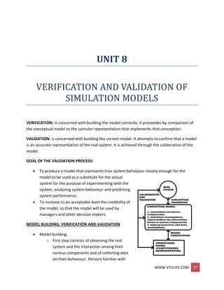
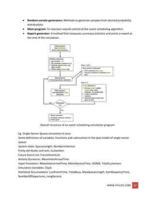
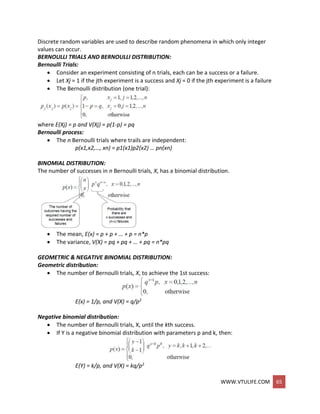
45. WWW.VTULIFE.COM 45
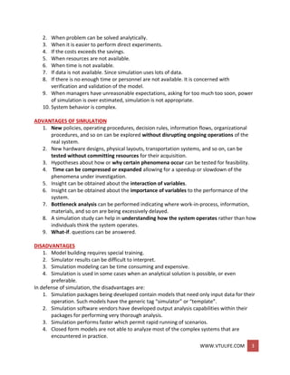
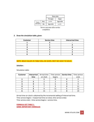
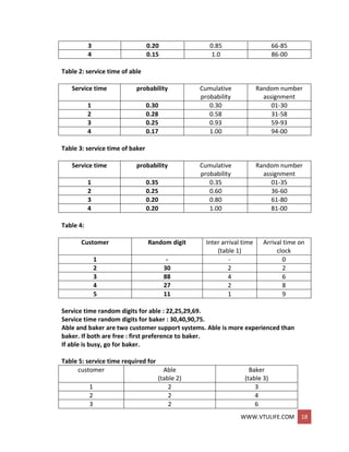
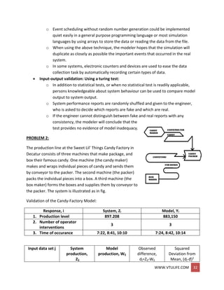
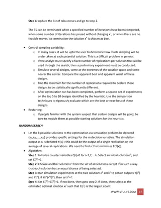
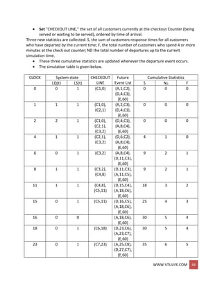
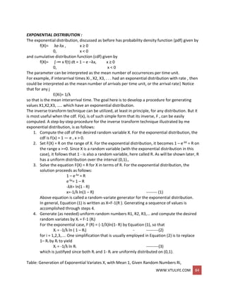
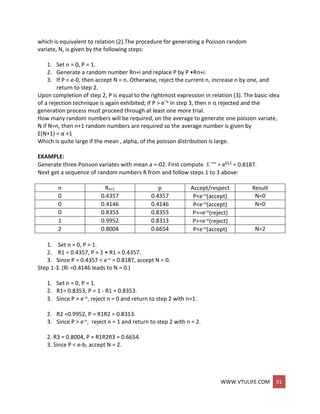
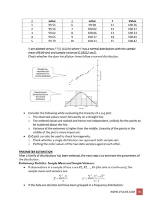
 Two statistics, server utilization and maximum queue length, will be collected.
 Server utilization is defined by total server busy time .(B) divided by total time(Te).
 Total busy time, B, and maximum queue length MQ, will be accumulated as the
simulation progresses.
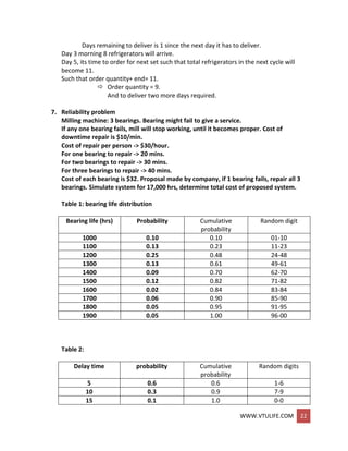
 As soon as the system snapshot at time CLOCK = 0 is complete, the simulation begins.
 At time 0, the imminent event is (D, 4).
 The CLOCK is advanced to time 4, and (D, 4) is removed from the FEL.
 Since LS(t) = 1 for 0 <= t <= 4 (i.e., the server was busy for 4 minutes), the cumulative
busy time is Increased from B = 0 to B = 4.
 By the event logic in Figure 1(B), set LS (4) = 0 (the server becomes idle).
 The FEL is left with only two future events, (A, 8) and (E, 0).
 The simulation CLOCK is next advanced to time 8 and an arrival event is executed.
 The simulation table covers interval [0,9].
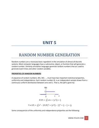
Simulation table for checkout counter:
Example: (The Checkout-Counter Simulation,
Continued)
Suppose the system analyst desires to estimate the mean response time and mean proportion
of customers who spend 4 or more minutes in the system the above mentioned model has to
be modified.
 Entities (Ci, t), representing customer Ci who arrived at time t.
 Event notices (A, t, Ci ), the arrival of customer Ci at future time t (D, f, Cj), the
departure of customer Cj at future time t.

46. WWW.VTULIFE.COM 46
 Set "CHECKOUT LINE," the set of all customers currently at the checkout Counter (being
served or waiting to be served), ordered by time of arrival.
Three new statistics are collected: S, the sum of customers response times for all customers
who have departed by the current time; F, the total number of customers who spend 4 or more
minutes at the check out counter; ND the total number of departures up to the current
simulation time.
 These three cumulative statistics are updated whenever the departure event occurs.
 The simulation table is given below.
CLOCK System state CHECKOUT
LINE
Future
Event List
Cumulative Statistics
LQ(t) LS(t) S ND F
0 0 1 (C1,0) (A,1,C2),
(D,4,C1),
(E,60)
0 0 0
1 1 1 (C1,0),
(C2,1)
(A,2,C3),
(D,4,C1),
(E,60)
0 0 0
2 2 1 (C1,0),
(C2,1),
(C3,2)
(D,4,C1),
(A,8,C4),
(E,60)
0 0 0
4 1 1 (C2,1),
(C3,2)
(D,6,C2),
(A,8,C4),
(E,60)
4 1 0
6 0 1 (C3,2) (A,8,C4),
(D,11,C3),
(E,60)
9 2 1
8 1 1 (C3,2),
(C4,8)
(D,11,C3),
(A,11,C5),
(E,60)
9 2 1
11 1 1 (C4,8),
(C5,11)
(D,15,C4),
(A,18,C6),
(E,60)
18 3 2
15 0 1 (C5,11) (D,16,C5),
(A,18,C6),
(E,60)
25 4 3
16 0 0 (A,18,C6),
(E,60)
30 5 4
18 0 1 (C6,18) (D,23,C6),
(A,23,C7),
(E,60)
30 5 4
23 0 1 (C7,23) (A,25,C8),
(D,27,C7),
(E,60)
35 6 5

47. WWW.VTULIFE.COM 47
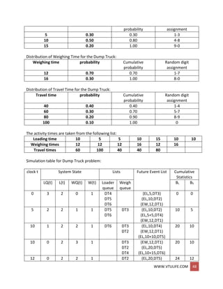
EXAMPLE: (THE DUMP TRUCK PROBLEM)
 Six dump truck are used to haul coal from the entrance of a small mine to the railroad.
 Each truck is loaded by one of two loaders.
 After loading, a truck immediately moves to scale, to be weighted as soon as possible.
 Both the loaders and the scale have a first come, first serve waiting line(or queue) for
trucks.
 The time taken to travel from loader to scale is considered negligible.
 After being weighted, a truck begins a travel time and then afterward returns to the
loader queue.
 The model has the following components:
o System state
[LQ(0, L(f), WQ(r), W(r)], where
LQ(f) = number of trucks in loader queue.
L(t) = number of trucks (0,1, or 2)being loaded.
WQ(t)= number of trucks in weigh queue.
W(t) = number of trucks (0 or 1) being weighed, all at simulation time t.
o Event notices
(ALQ,, t, DTi), dump truck arrives at loader queue
(ALQ) at time t
(EL, t, DTi), dump truck i ends loading (EL) at time t
(EW, t, DTi), dump truck i ends weighing (EW) at time t
o Entities The six dump trucks (DTI,..., DT6)
o Lists
Loader queue, all trucks waiting to begin loading, ordered on a first-
come, first-served basis Weigh queue, all trucks waiting to be weighed,
ordered on a first-come, first-serve basis.
o Activities Loading time, weighing time, and travel time.
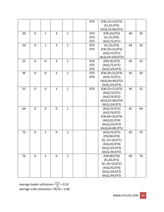
o Delays Delay at loader queue, and delay at scale. Distribution of Loading for the
Dump Truck.
Distribution of loading time for the dump trucks:
Loading time probability Cumulative Random digit

48. WWW.VTULIFE.COM 48
probability assignment
5 0.30 0.30 1-3
10 0.50 0.80 4-8
15 0.20 1.00 9-0
Distribution of Weighing Time for the Dump Truck:
Weighing time probability Cumulative
probability
Random digit
assignment
12 0.70 0.70 1-7
16 0.30 1.00 8-0
Distribution of Travel Time for the Dump Truck:
Travel time probability Cumulative
probability
Random digit
assignment
40 0.40 0.40 1-4
60 0.30 0.70 5-7
80 0.20 0.90 8-9
100 0.10 1.00 0
The activity times are taken from the following list:
Loading time 10 5 5 10 15 10 10
Weighing times 12 12 12 16 12 16
Travel times 60 100 40 40 80
Simulation table for Dump Truck problem:
clock t System State Lists Future Event List Cumulative
Statistics
LQ(t) L(t) WQ(t) W(t) Loader
queue
Weigh
queue
BL BS
0 3 2 0 1 DT4
DT5
DT6
(EL,5,DT3)
(EL,10,DT2)
(EW,12,DT1)
0 0
5 2 2 1 1 DT5
DT6
DT3 (EL,10,DT2)
(EL,5+5,DT4)
(EW,12,DT1)
10 5
10 1 2 2 1 DT6 DT3
DT2
(EL,10,DT4)
(EW,12,DT1)
(EL,10+10,DT5)
20 10
10 0 2 3 1 DT3
DT2
DT4
(EW,12,DT1)
(EL,20,DT5)
(EL,10+15,DT6)
20 10
12 0 2 2 1 DT2 (EL,20,DT5) 24 12

49. WWW.VTULIFE.COM 49
DT4 (EW,12+12,DT3)
(EL,25,DT6)
(ALQ,12+60,DT1)
20 0 1 3 1 DT2
DT4
DT5
(EW,24,DT3)
(EL,25,DT6)
(ALQ,72,DT1)
40 20
24 0 1 3 1 DT4
DT5
(EL,25,DT6)
(EW,24+12,DT2)
(ALQ,72,DT1)
(ALQ,24+100,DT3)
44 24
25 0 0 3 1 DT4
DT5
DT6
(EW,36,DT2)
(ALQ,72,DT1)
(ALQ,124,DT3)
45 25
36 0 0 2 1 DT5
DT6
(EW,36+16,DT4)
(ALQ,72,DT1)
(ALQ,36+40,DT2)
(ALQ,124,DT3)
45 36
52 0 0 1 1 DT6 (EW,52+12,DT5)
(ALQ,72,DT1)
(ALQ,76,DT2)
(ALQ,52+40,DT4)
(ALQ,124,DT3)
45 52
64 0 0 0 1 (ALQ,72,DT1)
(ALQ,76,DT2)
(EW,64+16,DT6)
(ALQ,92,DT4)
(ALQ,124,DT3)
(ALQ,64+80,DT5)
45 64
72 0 1 0 1 (ALQ,76,DT2)
(EW,80,DT6)
(EL,72+10,DT1)
(ALQ,92,DT4)
(ALQ,124,DT3)
(ALQ,144,DT5)
45 72
76 0 2 0 1 (EW,80,DT6)
(EL,82,DT1)
(EL,76+10,DT2)
(ALQ,92,DT4)
(ALQ,124,DT3)
(ALQ,144,DT5)
49 76
average loader utilization=
49/2
72
= 0.32
average scale utilization= 76/76 = 1.00

50. WWW.VTULIFE.COM 50
LIST PROCESSING
List processing deals with methods for handling lists of entities and the future event list.
LISTS: BASIC PROPERTIES AND OPERATIONS:
 Lists are a set of ordered or ranked records. In simulation, each record represents one
entity or one event notice.
 Since lists are ranked, they have a top or head (the first item on the list); some way to
traverse the list (to find the second, third, etc. items on the list); and a bottom or tail
(the last item on the list). A head pointer is a variable that points to or indicates the
record at the top of the list.
 An entity along with its attributes or an event notice will be referred to as a record. An
entity identifier and its attributes are fields in the entity record; the event type, event
time, and any other event-related data are fields in the event-notice record. Each record
on a list will also have a field that holds a “next pointer” that points to the next record
on the list. Some lists may also require a “previous pointer” to allow traversing the list
from bottom to top.
 The main operations on a list are:
o Removing a record from the top of the list.
o Removing a record from any location on the list.
o Adding an entity record to the top or bottom of the list.
o Adding a record to an arbitrary position on the list, determined by the ranking
rule.
USING ARRAYS FOR LIST PROCESSING
 Arrays are advantageous in that any specified record, say the i th, can be retrieved
quickly without searching, merely by referencing R(i ).
 Arrays are disadvantaged when items are added to the middle of a list or the list must
be rearranged. In addition, arrays typically have a fixed size, determined at compile
time.
 When using arrays for storing lists, there are two basic methods for keeping track of the
ranking of records in a list. One method is to store the first record in R(1), the second in
R(2), and so on, and the last in R(tailptr), where tailptr is used to refer to the last item in
the list. This method will be extremely inefficient for all except the shortest lists.
 In the second method, a variable called a head pointer, with name headptr, points to
the record at the top of the list. For example, if the record in position R(11) was the
record at the top of the list, then headptr would have a value of 11. In addition, each
record has a _eld that stores the index or pointer of the next record in the list. For
convenience, let R(i , next) represent the next index field.
 Example : (a list for the dump trucks at the weigh queue).
USING DYNAMIC ALLOCATION AND LINKED LISTS

51. WWW.VTULIFE.COM 51
 In procedural languages such as C and C++, and in most simulation languages, entity
records are dynamically created when an entity is created and event notice records are
dynamically created whenever an event is scheduled on the future event list.
 When an entity .dies..that is, exits from the simulated system and also after an event
occurs and the event notice is no longer needed, the corresponding records are freed.
 With dynamic allocation, a record is referenced by a pointer instead of an array index.
 If we want the third item on the list, we would have to traverse the list, counting items
until we reached the third record.
ADVANCED TECHNIQUES
 To speed up processing doubly-linked lists is to use a middle pointer in addition to a
head and tail pointer.
 The mid pointer will always point to the approximate middle of the list. when a new
record is being added to the list, the algorithm first examines the middle record to
decide whether to begin searching at the head of the list or the middle of the list.
 This technique should cut search times in half.
 Some advanced algorithms use list representations other than a doubly linked list, such
as heaps or trees.

52. WWW.VTULIFE.COM 52
SIMULATION SOFTWARE
CATEGORIES OF SIMULATION SOFTWARE
 General Purpose Languages
o C, C++, Java
 Simulation Languages
o GPSS, SIMAN, SLAM, SSF
 Simulation Environments
o Enterprise Dynamics, Arena, SIMUL8
FEATURES OF SIMULATION LANGUAGES
 Some focus on a single type of application.
 Built in features include:
o Statistics collection
o Time management
o Queue management
o Event generation
FEATURES OF SIMULATION ENVIRONMENTS
 Some focus on one type of application
 Icon based
 Analysis of I/O
 Advanced Statistics
 Optimization
 Support for Experimentation
HISTORY OF SIMULATION SOFTWARE (NANCE 1995)
 1955-60 Period of Search
 1961-65 Advent
 1966-70 Formative Period
 1971-78 Expansive Period
 1979-86 Period of Consolidation & Regeneration
 1987- 2008 Period of Integrated Environments

53. WWW.VTULIFE.COM 53
 2009 + The Future
THE SEARCH: 1955 – 60
 FORTRAN – one of a few languages.
 Focus on unifying concepts & reusable functions.
 General Simulation Program – first effort at “language” which as a set of functions.
THE ADVENT: 1961-65
 GPSS – 1961 @ IBM
o Based on block diagrams
o Well-suited for queuing models
o Expensive at first
 SIMSCRIPT – 1963 – Rand Corp.
o US Air Force – government is biggest user
o FORTRAN influence
o Owned by CACI in CA.
 GASP – 1961
o Based on Algol, then Fortran
o Collection of Fortran functions
 SIMULA – extension of Algol
o Widely used in Europe
 CSL (Control & Simulation Language)
FORMATIVE PERIOD: 1966-70
 Concepts caused major revisions of languages
 Languages gained wider usage
 GPSS (several variations)
 Simscript II – English-like
 ECSL – Europe
 SIMULA – added classes & inheritance
THE EXPANSION PERIOD: 1971-78
 GPSS/H – 1977
 GASP IV – 1974 – Purdue
 SIMULA
o Attempt to simplify the modeling process
o Program generators – severe limitations

54. WWW.VTULIFE.COM 54
CONSOLIDATION & REGENERATION: 1979-1986
 Movement to mini and PC computers
 SLAM II (descendant of GASP)
o 3 world views
o Event, Network, Continuous
 SIMAN (descendant of GASP)
o General Modeling + Block Diagrams
o 1st first major language - PC & MS-DOS
o Fortran functions w/ Fortran programming
INTEGRATED ENVIRONMENTS: 1987 – 2008
 Growth on PC’s
 Simulation Environments
o GUI
o Animation
o Data analyzers
THE FUTURE : 2009 – 2011
 Virtual Reality
 Improved Interfaces
 Better Animation
 Agent-based Modeling
SELECTION OF SIMULATION SOFTWARE
FEATURES:
Model-building features:
 Modeling worldview
 Input-data analysis capability
 Graphical model building
 Conditional routing
 Simulation programming
 Syntax
 Input flexibility
 Modeling conciseness
 Randomness
 Specialized components and templates
 User-built custom objects

55. WWW.VTULIFE.COM 55
 Continuous flow
 Interface with general programming language
Runtime environment:
 Execution speed
 Model size: number of variables and attributes
 Interactive debugger
 Model status and statistics
 Runtime license
Animation and layout features:
 Type of animation
 Import drawing and object files
 Dimension
 Movement
 Quality of motion
 Libraries of common objects
 Navigation
 Views
 Display step
 Selectable objects
 Hardware requirements
Output features:
 Scenario manager
 Run manager
 Warmup capability
 Independent replications
 Optimization
 Standardized reports
 Customized reports
 Statistical analysis
 Business graphics
 Costing module
 File export
 Database maintanence
Vendor support and Product Documentation:
 Training
 Documentation
 Help system

56. WWW.VTULIFE.COM 56
 Tutorials
 Support
 Upgrades, maintenance
 Track record
ADVICE FOR EVALUATING OR SELECTING SIMULATION SOFTWARE:
 Do not focus on a single issue, such as ease of use.
 Execution speed is important.
 Beware of advertising claims and demonstrations.
 Ask the vendor to solve a small version of your problem.
 Beware of “checklists” with “yes” and “no” as the entries.
 Simulation users ask whether the simulation model can link to and use the code or
routines written in external languages such as C,C++ or Java.
 There may be a significant trade-off between the graphical modl-building environments
and ones based on a simulation language.
Example Simulation: Checkout Counter – Single Server Queue
Consider at standard checkout counter environment with on clerk and one queue. Interarrival
times are exponentially distributed with mean 4.5 minutes; service times normally distributed
with mean 3.2 and standard deviation 0.6 minutes.
Simulation will run until 1000 customers are served.
SIMULATION IN JAVA
Java is widely used programming language that has been used extensively in simulation. It does
not provide any facilities directly aimed at aiding the simulation analyst, who therefore must
program all details of the event-scheduling/time-advance algorithm, the statistics-gathering
capability, the generation of samples from specified probability distributions, and the report
generator.
In java, all details must be explicitly programmed.
The following components are common to almost all models written in java:
 Clock: A variable defining simulated time.
 Initialization method: A method to define the system state at time 0.
 Min-time event method: A method that identifies the imminent event, that is, the
element of the future event list that has the smallest time-stamp.
 Event methods: For each event type, a method to update system state when that event
occurs.

57. WWW.VTULIFE.COM 57
 Random-variate generators: Methods to generate samples from desired probability
distributions.
 Main program: To maintain overall control of the event-scheduling algorithm.
 Report generator: A method that computes summary statistics and prints a report at
the end of the simulation.
Overall structure of an event scheduling simulation program
Eg: Single-Server Queue simulation in Java
Some definitions of variables, functions and subroutines in the java model of single server
queue:
System state: QueueLength, NumberInService
Entity attributes and sets: Customers
Future Event List: FutureEventList
Activity Durations: MeanInterArrivalTime
Input Prameters: MeanInterarrivalTime, MeanServiceTime, SIGMA, TotalCustomers
Simulation Variables: Clock
Statistical Accumulators: LastEventTime, TotalBusy, MaxQueueLength, SumResponseTime,
NumberOfDepartures, LongService

58. WWW.VTULIFE.COM 58
Summary Statistics: RHO=BusyTime/Clock, AVGR, PC4
FUNCTIONS:
Exponential(mu), normal(xmu, SIGMA)
METHODS:
Initialization, ProcessArrival, ProcessDeparture, ReportGeneration.
Java main program for the single-server queue simulation:
SIMULATION IN GPSS
General Purpose Simulation System

59. WWW.VTULIFE.COM 59
 Highly Structured, special purpose simulation programming language.
 Process Iteration Approach
 Queuing Systems
 Block Diagrams
o 40 standard blocks
o Block corresponds to a statement
 Transactions FLOW through the system
 Each entity has a name
o Name each queue, server, etc.
 In rectangle, parameters (as necessary)
 Right attachment, name of entity
 Far right column – GPSS Command
Diag: GPSS block diagram for the single server queue
simulation.
Eg: Single-server queue simulation in GPSS/H
 GENERATE block represents the arrival event.
 RVEXPO stands for “random variable exponentially
distributed”
 &IAT indicates that the mean time for the exponential
distribution comes from ampervariable &IAT.
 The next block is a QUEUE with a queue named
SYSTIME.
 The next QUEUE block (LINE) begins data collection for
the waiting line before the cashier.
 A customer captures the cashier, as represented by the
SEIZE block with the resource named CHECKOUT.
 The data collection for the waiting line statistics ends, as represented by the DEPART
block for the queue named LINE.
 The transaction service time at the cashier represented by an ADVANCE block.
 RVNORM indicates “random variable, normally distributed”.
 BLET block(LET) adds one to the account &COUNT.
 The escape route is to the block labeled TER.
 “**.**” indicates a value that may have two digits following the decimal point and up to
two before it.

60. WWW.VTULIFE.COM 60
GPSS Syntax (Assembly-type):
Label OpCode Subfields ; comment
 Label: col. 1, <= 9 alphanumeric, alpha start
 OpCode: 4+ characters of command
 Subfields: as necessary, separated by commas
 Comment: after ; or with * in column 1
GPSS Program:
Generate rvexpo (1,&IAT)
Queue Systime
Queue Line
Seize Checkout
Depart Line
Advance rvnorm(1,&mean,&stdev)
Release Checkout
Depart Systime
Test_GE M1, 4, Term
Blet &Count = &Count +1
Ter Terminate 1
Start &Limit

61. WWW.VTULIFE.COM 61
UNIT 3
STATISTICAL MODELS IN SIMULATION
The world the model-builder sees is probabilistic rather than deterministic.
 Some statistical model might well describe the variations. The world the model-builder
sees is probabilistic rather than deterministic.
 Some statistical model might well describe the variations.
An appropriate model can be developed by sampling the phenomenon of interest:
 Select a known distribution through educated guesses
 Make estimate of the parameter(s)
 Test for goodness of fit
REVIEW OF TERMINOLOGY AND CONCEPTS
DISCRETE RANDOM VARIABLES:
X is a discrete random variable if the number of possible values of X is finite, or countably
infinite.
Example: Consider jobs arriving at a job shop.
 Let X be the number of jobs arriving each week at a job shop.
 Rx = possible values of X (range space of X) = {0,1,2,…}
 p(xi) = probability the random variable is xi = P(X = xi)
p(xi), i = 1,2, … must satisfy:
The collection of pairs [xi, p(xi)], i = 1,2,…, is called the probability distribution of X, and p(xi) is
called the probability mass function (pmf) of X.
CONTINUOUS RANDOM VARIABLES:
X is a continuous random variable if its range space Rx is an interval or a collection of intervals.

62. WWW.VTULIFE.COM 62
 The probability that X lies in the interval [a,b] is given by:
 f(x), denoted as the pdf of X, satisfies:
 Properties:
 Example: Life of an inspection device is given by X, a continuous random variable with
pdf:
 X has an exponential distribution with mean 2 years
 Probability that the device’s life is between 2 and 3 years is:
CUMULATIVE DISTRIBUTION FUNCTION:
 Cumulative Distribution Function (cdf) is denoted by F(x), where F(x)= P(X <= x)

63. WWW.VTULIFE.COM 63
 Properties
o All probability question about X can be answered in terms of the cdf,
Eg:
 Example: An inspection device has cdf:
 The probability that the device lasts for less than 2 years:
 The probability that it lasts between 2 and 3 years:
EXPECTATION:
The expected value of X is denoted by E(X). The mean, m, or the 1st moment of X
 A measure of the central tendency
 The variance of X is denoted by V(X) or var(X) or σ2
The variance of X is denoted by V(X) or var(X) or σ2
 Definition: V(X) = E[(X – E[X]2]
 Also, V(X) = E(X2) – [E(x)]2
 A measure of the spread or variation of the possible values of X around the mean
The standard deviation of X is denoted by σ
 Definition: square root of V(X)
 Expressed in the same units as the mean
Example: The mean of life of the previous inspection device is:
To compute variance of X, we first compute E(X2):
Hence, the variance and standard deviation of the device’s life are:
USEFUL STATISTICAL MODELS

64. WWW.VTULIFE.COM 64
Statistical models appropriate to some application areas. The areas include:
 Queueing systems
 Inventory and supply-chain systems
 Reliability and maintainability
 Limited data
QUEUEING SYSTEMS:
 In a queueing system, interarrival and service-time patterns can be probabilistic.
 Sample statistical models for interarrival or service time distribution:
o Exponential distribution: if service times are completely random.
o Normal distribution: fairly constant but with some random variability (either
positive or negative)
o Truncated normal distribution: similar to normal distribution but with restricted
value.
o Gamma and Weibull distribution: more general than exponential (involving
location of the modes of pdf’s and the shapes of tails.)
INVENTORY AND SUPPLY CHAIN:
 In realistic inventory and supply-chain systems, there are at least three random
variables:
o The number of units demanded per order or per time period
o The time between demands
o The lead time
 Sample statistical models for lead time distribution:
o Gamma
 Sample statistical models for demand distribution:
o Poisson: simple and extensively tabulated.
o Negative binomial distribution: longer tail than Poisson (more large demands).
o Geometric: special case of negative binomial given at least one demand has
occurred.
RELIABILITY AND MAINTAINABILITY:
Time to failure (TTF)
 Exponential: failures are random
 Gamma: for standby redundancy where each component has an exponential TTF
 Weibull: failure is due to the most serious of a large number of defects in a system of
components.
 Normal: failures are due to wear
OTHER AREAS:
For cases with limited data, some useful distributions are:
 Uniform, triangular and beta
Other distribution:
 Bernoulli, binomial and Hyper exponential.
DISCRETE DISTRIBUTIONS

65. WWW.VTULIFE.COM 65
Discrete random variables are used to describe random phenomena in which only integer
values can occur.
BERNOULLI TRIALS AND BERNOULLI DISTRIBUTION:
Bernoulli Trials:
 Consider an experiment consisting of n trials, each can be a success or a failure.
 Let Xj = 1 if the jth experiment is a success and Xj = 0 if the jth experiment is a failure
 The Bernoulli distribution (one trial):
where E(Xj) = p and V(Xj) = p(1-p) = pq
Bernoulli process:
 The n Bernoulli trials where trails are independent:
p(x1,x2,…, xn) = p1(x1)p2(x2) … pn(xn)
BINOMIAL DISTRIBUTION:
The number of successes in n Bernoulli trials, X, has a binomial distribution.
 The mean, E(x) = p + p + … + p = n*p
 The variance, V(X) = pq + pq + … + pq = n*pq
GEOMETRIC & NEGATIVE BINOMIAL DISTRIBUTION:
Geometric distribution:
 The number of Bernoulli trials, X, to achieve the 1st success:
E(x) = 1/p, and V(X) = q/p2
Negative binomial distribution:
 The number of Bernoulli trials, X, until the kth success.
 If Y is a negative binomial distribution with parameters p and k, then:
E(Y) = k/p, and V(X) = kq/p2

66. WWW.VTULIFE.COM 66
POISSON DISTRIBUTION:
Poisson distribution describes many random processes quite well and is mathematically quite
simple where α > 0, pdf and cdf are:
E(X) = α = V(X)
Example: A computer repair person is “beeped” each time there is a call for service. The
number of beeps per hour ~ Poisson(α = 2 per hour).
 The probability of three beeps in the next hour:
p(3) = e-2 23 /3! = 0.18
also, p(3) = F(3) – F(2) = 0.857-0.677=0.18
 The probability of two or more beeps in a 1-hour period:
p(2 or more) = 1 – p(0) – p(1)
= 1 – F(1)
= 0.594
CONTINUOUS DISTRIBUTIONS
Continuous random variables can be used to describe random phenomena in which the variable
can take on any value in some interval.
UNIFORM DISTRIBUTION:
A random variable X is uniformly distributed on the interval (a,b), U(a,b), if its pdf and cdf are:
Properties:
 P(x1 < X < x2) is proportional to the length of the interval [F(x2) – F(x1) = (x2-x1)/(b-a)]
 E(X) = (a+b)/2 V(X) = (b-a)2/12

67. WWW.VTULIFE.COM 67
 U(0,1) provides the means to generate random numbers, from which random variates
can be generated.
EXPONENTIAL DISTRIBUTION:
A random variable X is exponentially distributed with parameter λ > 0 if its pdf and cdf are:
E(X) = 1/λ V(X) = 1/λ2
 Used to model interarrival times when arrivals are completely random, and to model
service times that are highly variable
 For several different exponential pdf’s (see figure), the value of intercept on the vertical
axis is λ, and all pdf’s eventually intersect.
 Memoryless property
o For all s and t greater or equal to 0:
P(X > s+t | X > s) = P(X > t)
o Example: A lamp ~ exp(λ = 1/3 per hour), hence, on average, 1 failure per 3 hours.
The probability that the lamp lasts longer than its mean life is:
P(X > 3) = 1-(1-e-3/3 ) = e-1 = 0.368
o The probability that the lamp lasts between 2 to 3 hours is:
P(2 <= X <= 3) = F(3) – F(2) = 0.145
o The probability that it lasts for another hour given it is operating for 2.5 hours:
P(X > 3.5 | X > 2.5) = P(X > 1) = e-1/3 = 0.717
NORMAL DISTRIBUTION:
A random variable X is normally distributed has the pdf:
Mean: −∞ < μ < ∞
Variance: σ2 > 0
Denoted as X ~ N(μ,σ2 )

68. WWW.VTULIFE.COM 68
Special properties:
f(μ-x)=f(μ+x); the pdf is symmetric about μ.
 The maximum value of the pdf occurs at x = μ; the mean and mode are equal.
Evaluating the distribution:
 Use numerical methods (no closed form)
 Independent of μ and σ, using the standard normal distribution:
Z ~ N(0,1)
 Transformation of variables: let Z = (X - μ) / σ,
 Example: The time required to load an oceangoing vessel, X, is distributed as N(12,4)
The probability that the vessel is loaded in less than 10 hours:
 Using the symmetry property, Φ(1) is the complement of Φ (-1)
WEIBULL DISTRIBUTION:
A random variable X has a Weibull distribution if its pdf has the form:
3 parameters:
 Location parameter: υ, (−∞ <ν < ∞)
 Scale parameter: β , (β > 0)
 Shape parameter. α, (> 0)
Example: υ = 0 and α = 1:

69. WWW.VTULIFE.COM 69
LOGNORMAL DISTRIBUTION:
A random variable X has a lognormal distribution if its pdf has the form:
Mean E(X) = eμ+σ2 /2
 Variance V(X) = e2+2 (e2-1)
Relationship with normal distribution
 When Y ~ N(μ, σ2 ), then X = eY ~ lognormal(μ, σ2)
 Parameters μ and σ2 are not the mean and variance of the Lognormal.
POISSON DISTRIBUTION
Definition: N(t) is a
counting function that
represents the number
of events occurred in
[0,t].
A counting process {N(t),
t>=0} is a Poisson

70. WWW.VTULIFE.COM 70
process with mean rate λ if:
 Arrivals occur one at a time
 {N(t), t>=0} has stationary increments
 {N(t), t>=0} has independent increments
Properties:
 Equal mean and variance: E[N(t)] = V[N(t)] = λt
 Stationary increment: The number of arrivals in time s to t is also Poisson-distributed
with mean λ(t-s)
INTERARRIVAL TIMES:
Consider the interarrival times of a Possion process (A1, A2, …), where Ai is the elapsed time
between arrival i and arrival i+1
The 1st arrival occurs after time t iff there are no arrivals in the interval [0,t], hence:
 P{A1 > t} = P{N(t) = 0} = e-t
 P{A1 <= t} = 1 – e-t [cdf of exp(λ)]
Interarrival times, A1, A2, …, are exponentially distributed and independent with mean 1/λ.
SPLITTING AND POOLING:
Splitting:
 Suppose each event of a Poisson process can be classified as Type I, with probability p
and Type II, with probability 1-p.
 N(t) = N1(t) + N2(t), where N1(t) and N2(t) are both Poisson processes with rates λ p and
λ (1-p).
Pooling:
 Suppose two Poisson processes are pooled together
 N1(t) + N2(t) = N(t), where N(t) is a Poisson processes with rates λ1 + λ2
NONSTATIONARY POISSON PROCESS (NSPP):
Poisson Process without the stationary increments, characterized by λ(t), the arrival rate at
time t.

71. WWW.VTULIFE.COM 71
 The expected number of arrivals by time t, Λ(t):
Relating stationary Poisson process n(t) with rate λ=1 and NSPP N(t) with rate λ(t):
 Let arrival times of a stationary process with rate λ = 1 be t1, t2, …, and arrival times of a
NSPP with rate λ(t) be T1, T2, …, we know:
ti = Λ(Ti)
Ti = Λ−1(ti)
Example: Suppose arrivals to a Post Office have rates 2 per minute from 8 am until 12 pm, and
then 0.5 per minute until 4 pm.
 Let t = 0 correspond to 8 am, NSPP N(t) has rate function:
 Expected number of arrivals by time t:
Hence, the probability distribution of the number of arrivals between 11 am and 2 pm.
P[N(6) – N(3) = k] = P[N(Λ(6)) – N(Λ(3)) = k]
= P[N(9) – N(6) = k]
= e(9-6) (9-6)k /k! = e3 (3)k /k!
EMPIRICAL DISTRIBUTIONS:
 A distribution whose parameters are the observed values in a sample of data.
 May be used when it is impossible or unnecessary to establish that a random variable
has any particular parametric distribution.
 Advantage: no assumption beyond the observed values in the sample.
 Disadvantage: sample might not cover the entire range of possible values.
PROBLEMS
1. A recent survey indicated that 82% of single women aged 25 years old will be married
in their lifetime. Using the binomial distribution, find the probability that two or three
women in a sample of twenty will never get married.
Solution:
Let X be defined as the number of women in the sample never married
P(2 <= X <= 3) = p(2) + p(3)
=20C2 * (.82)(20-2) * (1-.82)2 + 20C3 * (.18)3 * (.82)20-3
=
20!
(20−2)!2!
* (0.82)18 * (0.18)2 +
20!
(20−3)!3!
* (0.82)17 * (0.18)3
=0.173 + 0.228 = 0.401
=40.1%