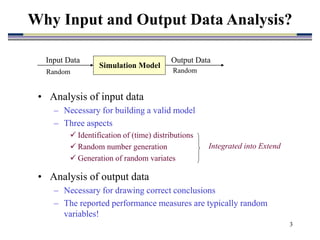
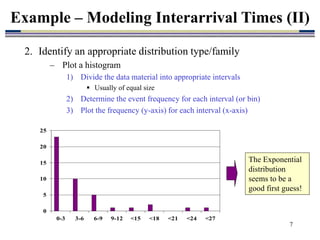
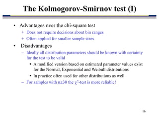
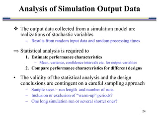
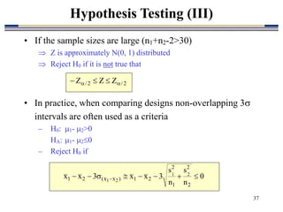
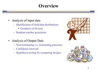
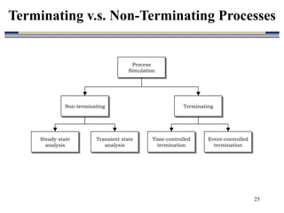
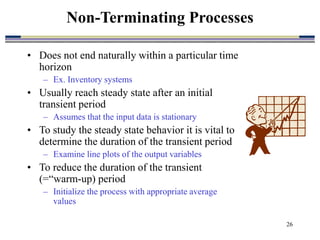
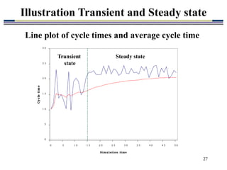
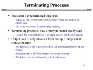
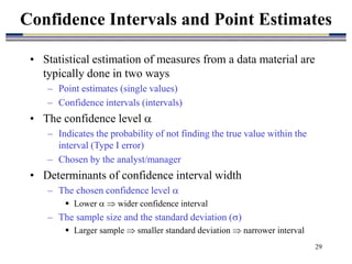
1. Input and output data analysis is necessary for building a valid simulation model and drawing correct conclusions from the model. 2. Key aspects of input data analysis include identifying appropriate time distributions from field data, generating random numbers, and producing random variates. Output data analysis considers non-terminating vs terminating processes, confidence intervals, and hypothesis testing for model comparisons. 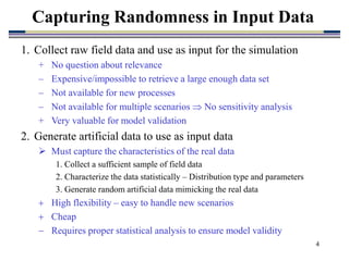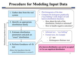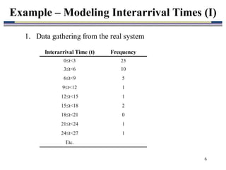3. Common procedures for modeling input data include collecting field data, identifying a plausible distribution, estimating distribution parameters, and performing goodness-of-fit tests to validate the chosen distribution. Artificial data can also be generated if real data is unavailable or limited.

1. 1
Simulation Input and
Output Data Analysis
Chapter 9
Business Process Modeling, Simulation and
Design
Augmented with material from other sources

2. 2
Overview
• Analysis of input data
– Identification of field data distributions
 Goodness-of-fit tests
 Random number generation
• Analysis of Output Data
– Non-terminating v.s. terminating processes
– Confidence intervals
– Hypothesis testing for comparing designs

3. 3
• Analysis of input data
– Necessary for building a valid model
– Three aspects
 Identification of (time) distributions
 Random number generation
 Generation of random variates
Why Input and Output Data Analysis?
• Analysis of output data
– Necessary for drawing correct conclusions
– The reported performance measures are typically random
variables!
Integrated into Extend
Simulation Model
Output Data
Input Data
Random Random

4. 4
1. Collect raw field data and use as input for the simulation
+ No question about relevance
– Expensive/impossible to retrieve a large enough data set
– Not available for new processes
– Not available for multiple scenarios  No sensitivity analysis
+ Very valuable for model validation
2. Generate artificial data to use as input data
 Must capture the characteristics of the real data
1. Collect a sufficient sample of field data
2. Characterize the data statistically – Distribution type and parameters
3. Generate random artificial data mimicking the real data
 High flexibility – easy to handle new scenarios
 Cheap
 Requires proper statistical analysis to ensure model validity
Capturing Randomness in Input Data

5. 5
• Plot histograms of the data
• Compare the histogram graphically
(“eye-balling”) with shapes of well
known distribution functions
– How about the tails of the
distribution, limited or unlimited?
– How to handle negative outcomes?
Procedure for Modeling Input Data
4. Perform Goodness–of–fit
test
(Reject the hypothesis that the
picked distribution is correct?)
Distribution
hypothesis
rejected
1. Gather data from the real
system
2. Identify an appropriate
distribution family
3. Estimate distribution
parameters and pick an
“exact” distribution
• Informal test – “eye-balling”
• Formal tests, for example
– 2 - test
– Kolmogorov-Smirnov test
If a known distribution can not be accepted
 Use an empirical distribution

6. 6
1. Data gathering from the real system
Example – Modeling Interarrival Times (I)
Interarrival Time (t) Frequency
0t<3 23
3t<6 10
6t<9 5
9t<12 1
12t<15 1
15t<18 2
18t<21 0
21t<24 1
24t<27 1
Etc.

7. 7
2. Identify an appropriate distribution type/family
– Plot a histogram
1) Divide the data material into appropriate intervals
 Usually of equal size
2) Determine the event frequency for each interval (or bin)
3) Plot the frequency (y-axis) for each interval (x-axis)
Example – Modeling Interarrival Times (II)
0
5
10
15
20
25
0-3 3-6 6-9 9-12 <15 <18 <21 <24 <27
The Exponential
distribution
seems to be a
good first guess!

8. 8
3. Estimate the parameters defining the chosen
distribution
– In the current example Exp() has been chosen  need to
estimate the parameter 
 ti = the ith interarrival time in the collected sample of n
observations
Example – Modeling Interarrival Times (III)
084
.
0
...
t
1
N
t
t
1
N
1
i
i











9. 9
4. Perform Goodness-of-fit test
– The purpose is to test the hypothesis that the data material is
adequately described by the “exact” distribution chosen in steps 1-
3.
– Two of the most well known standardized tests are
• The 2-test
– Should not be applied if the sample size n<20
• The Kolmogorov-Smirnov test
– A relatively simple but imprecise test
– Often used for small sample sizes
– The 2-test will be applied for the current example
Example – Modeling Interarrival Times (III)

10. 10
 In principle
 A statistical test comparing the relative frequencies for the
intervals/bins in a histogram with the theoretical probabilities of
the chosen distribution
• Assumptions
– The distribution involves k parameters estimated from the sample
– The sample contains n observations (sample size=n)
– F0(x) denotes the chosen/hypothesized CDF
Performing a 2-Test (I)
Data: x1, x2, …, xn
(n observations from the real
system)
Model: X1, X2,…, Xn
(Random variables, independent and
identically distributed with CDF F(x))
Null hypothesis H0: F(x) = F0(x)
Alternative hypothesis HA: F(x)  F0(x)

11. 11
Performing a 2-Test (II)
1. Take the entire data range and divide it into r non
overlapping intervals or bins
• pi = The probability that an observation X belongs to bin i
 The Null Hypothesis  pi = F0(ai) - F0(ai-1)
• To improve the accuracy of the test
– choose the bins (intervals) so that the probabilities pi (i=1,2, …r)
are equal for all bins
The area = p2 = F0(a2) - F0(a1)
Data values
Min=a0 a1 a2 ar-1 ar=Max
…
a3 ar-2
Bin: 1 2 3 r-1 r
f0(x)

12. 12
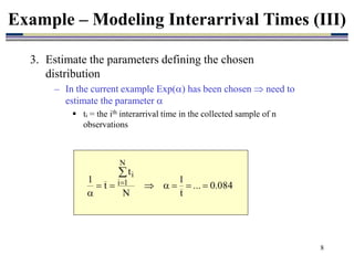
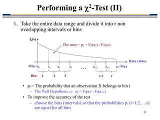
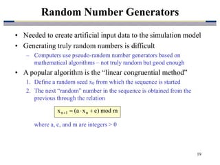
2. Define r random variables Oi, i=1, 2, …r
– Oi=number of observations in bin i (= the interval (ai-1, ai])
– If H0 is true  the expected value of Oi = n*pi
• Oi is Binomially distributed with parameters n and pi
3. Define the test variable T
Performing a 2-Test (III)
 

 



r
1
i i
2
i
i
p
n
p
n
O
T
– If H0 is true  T follows a 2(r-k-1) distribution
– T = The critical value of T corresponding to a significance level 
obtained from a 2(r-k-1) distribution table
– Tobs = The value of T computed from the data material
 If Tobs > T  H0 can be rejected on the significance level 

13. 13
• Depends on the sample size n and on the bin selection (the
size of the intervals)
• Rules of thumb
– The 2-test is acceptable for ordinary significance levels (=1%,
5%) if the expected number of observations in each interval is
greater than 5 (n*pi>5 for all i)
– In the case of continuous data and a bin selection such that pi is
equal for all bins 
 n20  Do not use the 2-test
 20<n 50  5-10 bins recommendable
 50<n 100  10-20 bins recommendable
 n >100  n0.5 – 0.2n bins recommendable
Validity of the 2-Test

14. 14
• Hypothesis – the interarrival time Y is Exp(0.084) distributed
H0: YExp(0.084)
HA: YExp(0.084)
• Bin sizes are chosen so that the probability pi is equal for all r
bins and n*pi>5 for all i
– Equal pi  pi=1/r
– n*pi>5  n/r > 5  r<n/5
– n=50  r<50/5=10  Choose for example r=8  pi=1/8
• Determining the interval limits ai, i=0,1,…8
Example – Modeling Interarrival Times (IV)
i
a
*
084
.
0
i
0 e
1
)
a
(
F
H 



084
.
0
)
p
*
i
1
ln(
a
e
1
p
*
i i
i
a
*
084
.
0
i
i






 
i=1  a1=ln(1-(1/8))/(-0.084)=1.590
i=2  a2=ln(1-(2/8))/(-0.084)=3.425

i=8  a8 =ln(1-(8/8))/(-0.084)=

15. 15
• Determining the critical value T
– If H0 is true  T2(8-1-1)=2(6)
– If =0.05  P(T T0.05)=1-=0.95  /2 table/  T0.05=12.60
• Rejecting the hypothesis
– Tobs=39.6>12.6= T0.05
 H0 is rejected on the 5% level
Example – Modeling Interarrival Times (V)
 
6
.
39
8
/
50
8
/
50
o
T
8
1
i
2
i
obs 

 

Note:
oi = the actual number of
observations in bin i
• Computing the test statistic Tobs

16. 16
• Advantages over the chi-square test
+ Does not require decisions about bin ranges
+ Often applied for smaller sample sizes
• Disadvantages
– Ideally all distribution parameters should be known with certainty
for the test to be valid
 A modified version based on estimated parameter values exist
for the Normal, Exponential and Weibull distributions
 In practice often used for other distributions as well
– For samples with n30 the 2-test is more reliable!
The Kolmogorov-Smirnov test (I)

17. 17
• Compares an empirical “relative-frequency” CDF with the
theoretical CDF (F(x)) of a chosen (hypothesized) distribution
– The empirical CDF = Fn(x) = (number of xix)/n
 n=number of observations in the sample
 xi=the value of the ith smallest observation in the sample
 Fn(xi)=i/n
• Procedure
1. Order the sample data from the smallest to the largest value
2. Compute D+ , D– and D = max{D+ , D–}
3. Find the tabulated critical KS value corresponding to the sample size n
and the chosen significance level, 
4. If the critical KS value  D  reject the hypothesis that F(x) describes
the data material’s distribution
The Kolmogorov-Smirnov test (II)





 




)
x
(
F
n
i
max
D i
n
i
1 




 





n
1
i
)
x
(
F
max
D i
n
i
1

18. 18
• Common situation especially when designing new processes
– Try to draw on expert knowledge from people involved in similar tasks
 When estimates of interval lengths are available
– Ex. The service time ranges between 5 and 20 minutes
Plausible to use a Uniform distribution with min=5 and max=20
 When estimates of the interval and most likely value exist
– Ex. min=5, max=20, most likely=12
Plausible to use a Triangular distribution with those parameter values
 When estimates of min=a, most likely=c, max=b and the
average value=x-bar are available
Use a -distribution with parameters  and 
Distribution Choice in Absence of Sample Data
)
a
b
)(
x
c
(
)
b
a
c
2
)(
a
x
(







 
)
a
x
(
x
b






19. 19
• Needed to create artificial input data to the simulation model
• Generating truly random numbers is difficult
– Computers use pseudo-random number generators based on
mathematical algorithms – not truly random but good enough
• A popular algorithm is the “linear congruential method”
1. Define a random seed x0 from which the sequence is started
2. The next “random” number in the sequence is obtained from the
previous through the relation
where a, c, and m are integers > 0
Random Number Generators
m
mod
)
c
x
a
(
x n
1
n 




20. 20
• Assume that m=8, a=5, c=7 and x0=4
Example – The Linear Congruential Method
8
mod
)
7
x
5
(
x n
1
n 


 
n xn 5xn+7 (5xn+7)/8 xn+1
0 4 27 3 + 3 /8 3
1 3 22 2 + 6 /8 6
2 6 37 4 + 5 /8 5
3 5 32 4 + 0 /8 0
4 0 7 0 + 7 /8 7
5 7 42 5 + 2 /8 2
6 2 17 2 + 1 /8 1
7 1 12 1 + 4 /8 4
Larger m  longer sequence before it starts repeating itself

21. 21
• Test for detecting dependencies in a sequence of generated
random numbers
• A run is defined as a sequence of increasing or decreasing
numbers
– “+” indictes an increasing run
– “–” indicates a decreasing run
The Runs Test (I)
Ex. Numbers: 1, 7, 8, 6, 5, 3, 4, 10, 12, 15
runs: + + – – – + + + + +
• The test is based on comparing the number of runs in a true
random sequence with the number of runs in the observed
sequence

22. 22
• Hypothesis: H0: Sequence of numbers is independent
HA: Sequence of numbers is not independent
• R = # runs in a truly random sequence of n numbers (random
variable)
• Have been shown that…
The Runs Test (II)
R=(2n-1)/3
Test statistic: Z={(R-R)/R}N(0,1)
R=(16n-29)/90 RN(R, R)
• Assuming: confidence level  and a two sided test
– P(-Z/2ZZ/2)=1-
– H0 is rejected if Zobserved> Z/2

23. 23
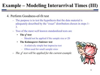
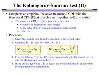
• Assume random numbers, r, from a Uniform (0, 1) distribution
are available
 Random numbers from any distribution can be obtained by applying the
“inverse transformation technique”
The inverse Transformation Technique
1. Generate a U[0, 1] distributed random number r
2. T is a random variable with a CDF FT(t) from which we would
like to obtain a sequence of random numbers
– Note: 0 FT(t) 1 for all values of t
Generating Random Variates
)
r
(
F
t
t
for
solve
and
r
)
t
(
F
Let 1
T
T




 t is a random number from the distribution of T, i.e., a realization of T

24. 24
 The output data collected from a simulation model are
realizations of stochastic variables
– Results from random input data and random processing times
 Statistical analysis is required to
1. Estimate performance characteristics
– Mean, variance, confidence intervals etc. for output variables
2. Compare performance characteristics for different designs
• The validity of the statistical analysis and the design
conclusions are contingent on a careful sampling approach
– Sample sizes – run length and number of runs.
– Inclusion or exclusion of “warm-up” periods?
– One long simulation run or several shorter ones?
Analysis of Simulation Output Data

25. 25
Process
Simulation
Process
Simulation
Terminating
Terminating
Non-terminating
Non-terminating
Event-controlled
termination
Event-controlled
termination
Time-controlled
termination
Time-controlled
termination
Transient state
analysis
Transient state
analysis
Steady state
analysis
Steady state
analysis
Process
Simulation
Process
Simulation
Terminating
Terminating
Non-terminating
Non-terminating
Event-controlled
termination
Event-controlled
termination
Time-controlled
termination
Time-controlled
termination
Transient state
analysis
Transient state
analysis
Steady state
analysis
Steady state
analysis
Terminating v.s. Non-Terminating Processes

26. 26
• Does not end naturally within a particular time
horizon
– Ex. Inventory systems
• Usually reach steady state after an initial
transient period
– Assumes that the input data is stationary
• To study the steady state behavior it is vital to
determine the duration of the transient period
– Examine line plots of the output variables
• To reduce the duration of the transient
(=“warm-up) period
– Initialize the process with appropriate average
values
Non-Terminating Processes

27. 27
Illustration Transient and Steady state
0
5
1 0
1 5
2 0
2 5
3 0
0 5 1 0 1 5 2 0 2 5 3 0 3 5 4 0 4 5 5 0
Simulation time
Cy
cle
tim
e
Line plot of cycle times and average cycle time
Transient
state
Steady state

28. 28
• Ends after a predetermined time span
– Typically the system starts from an empty state and ends in an
empty state
– Ex. A grocery store, a construction project, …
• Terminating processes may or may not reach steady state
– Usually the transient period is of great interest for these processes
• Output data usually obtained from multiple independent
simulation runs
– The length of a run is determined by the natural termination of the
process
– Each run need a different stream of random numbers
– The initial state of each run is typically the same
Terminating Processes

29. 29
• Statistical estimation of measures from a data material are
typically done in two ways
– Point estimates (single values)
– Confidence intervals (intervals)
• The confidence level 
– Indicates the probability of not finding the true value within the
interval (Type I error)
– Chosen by the analyst/manager
• Determinants of confidence interval width
– The chosen confidence level 
 Lower   wider confidence interval
– The sample size and the standard deviation ()
 Larger sample  smaller standard deviation  narrower interval
Confidence Intervals and Point Estimates

30. 30
• In simulation the most commonly used statistics are the
mean and standard deviation ()
– From a sample of n observations
Point estimate of the mean:
Point estimate of  :
Important Point Estimates
n
x
...
x
x
x n
2
1 



1
n
)
x
x
(
s
n
1
i
2
i






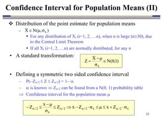
31. 31
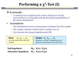
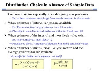
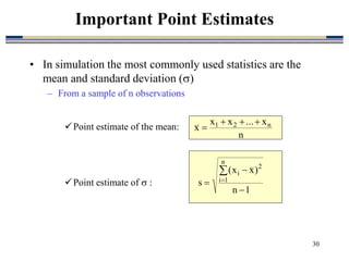
 Characteristics of the point estimate for the population mean
– Xi = Random variable representing the value of the ith observation in a
sample of size n, (i=1, 2, …, n)
– Assume that all observations Xi are independent random variables
– The population mean = E[Xi]=
– The population standard deviation=(Var[Xi])0.5=
– Point estimate of the population mean=
– Mean and Std. Dev. of the point estimate for the population mean
Confidence Interval for Population Means (I)
n
X
X
X
X n
2
1 




        








n
n
n
X
E
X
E
X
E
X
E n
2
1 
n
n
n
n
)
X
(
Var
)
X
(
Var
)
X
(
Var 2
2
2
2
1
x










32. 32
 For any distribution of Xi (i=1, 2, …n), when n is large (n30), due
to the Central Limit Theorem
 If all Xi (i=1, 2, …n) are normally distributed, for any n
• A standard transformation:
Confidence Interval for Population Means (II)
)
,
(
N
X x



)
1
,
0
(
N
X
Z
x





x
2
/
x
2
/
2
/
x
2
/ Z
x
Z
x
Z
x
Z 














 



• Defining a symmetric two sided confidence interval
– P(Z/2  Z  Z/2) = 1 
–  is known  Z/2 can be found from a N(0, 1) probability table
 Confidence interval for the population mean 
 Distribution of the point estimate for population means
–

33. 33
• In case  is unknown we need to estimate it
– Use the point estimate s
 The test variable Z is no longer Normally distributed, it follows a
Students-t distribution with n-1 degrees of freedom

Confidence Interval for Population Means (III)
x
2
/
x
2
/ Z
x
Z
x 







 

n
x 


n
s
t
x
n
s
t
x 2
/
),
1
n
(
2
/
),
1
n
( 





 



In practice when n is large (30) the t-distribution is
often approximated with the Normal distribution!
• In case the population standard deviation, , is known

34. 34
• A common problem in simulation
– How many runs and how long should they be?
• Depends on the variability of the sought output variables
• If a symmetric confidence interval of width 2d is desired
for a mean performance measure 

Determining an Appropriate Sample Size
d
x
d
x 




 2
2
/
2
/ d
/
)
Z
(
n
n
/
)
Z
(
d 
 






 2
2
/ d
/
)
Z
s
(
n 


 If  is unknown and estimated with s

– If x-bar is normally distributed


35. 35
1. Testing if a population mean () is equal to, larger
than or smaller than a given value
– Suppose that in a sample of n observations the point estimate of =
Hypothesis Testing (I)
x
Hypothesis Reject H0 if … Type of test
H0: =a Symmetric two tail
test
HA: a
H0: a One tail test
HA: <a
H0: a One tail test
HA: >a
or
Z
n
/
s
a
x
2
/




2
/
Z
n
/
s
a
x







Z
n
/
s
a
x



Z
n
/
s
a
x

36. 36
2. Testing if two sample means are significantly different
– Useful when comparing process designs
• A two tail test when 1=2=s
– H0: 1- 2=a /typically a=0/
HA: 1- 2a
– The test statistic Z belongs to a Student-t distribution
– Reject H0 on the significance level  if it is not true that
Hypothesis Testing (II)
)
2
n
n
(
t
n
1
n
1
s
)
(
x
x
Z 2
1
2
1
2
1
2
1










)
2
/
1
(
),
2
n
n
(
)
2
/
1
(
),
2
n
n
( 2
1
2
1
t
Z
t 






 



37. 37
• If the sample sizes are large (n1+n2-2>30)
 Z is approximately N(0, 1) distributed
 Reject H0 if it is not true that
Hypothesis Testing (III)
2
/
2
/ Z
Z
Z 
 


0
n
s
n
s
3
x
x
3
x
x
2
2
1
2
2
1
)
x
x
(
2
1
2
1
2
1







 
• In practice, when comparing designs non-overlapping 3
intervals are often used as a criteria
– H0: 1- 2>0
HA: 1- 20
– Reject H0 if