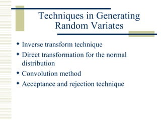
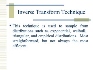
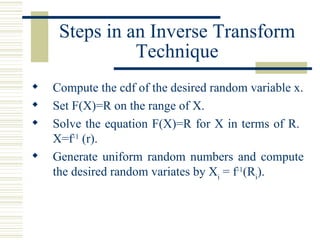
The document discusses random variate generation, detailing various techniques such as inverse transform, direct transformation for the normal distribution, convolution method, and acceptance-rejection technique. It explains how to generate random variates from specific distributions, including exponential and triangular distributions. Additionally, it outlines steps for sampling and analyzing simulation data, including data collection and goodness-of-fit tests.

1. RANDOM VARIATE
GENERATION
Chapter 9

2. Random Variate
 A value being sampled from a proven
distribution of an input variable.
 Examples such as inter-arrival time and
service time.
 RV generators – techniques used to generate
random variates.

3. Techniques in Generating
Random Variates
 Inverse transform technique
 Direct transformation for the normal
distribution
 Convolution method
 Acceptance and rejection technique

4. Inverse Transform Technique
 This technique is used to sample from
distributions such as exponential, weibull,
triangular, and empirical distributions. Most
straightforward, but not always the most
efficient.

5. Steps in an Inverse Transform
Technique
 Compute the cdf of the desired random variable x.
 Set F(X)=R on the range of X.
 Solve the equation F(X)=R for X in terms of R.
X=f-1
(r).
 Generate uniform random numbers and compute
the desired random variates by Xi
= f-1
(Ri
).

6. Derivation of RV generator for
an exponential distribution
Ex. Given exponential distribution,
Thus, the Random Variate Generator is
f x
e x
otherwise
x
( )
,
,
=
≥





1
0
0
1
β
β
x R
or
x R
i i
i i
= −
=
β
β
ln( )
ln( )
1

7. Uniform Distribution
Thus, the RVG is
f x b a
a x b
otherwise
( )
,
,
= −
≤ ≤




1
0
x a b a Ri i= + −( )

8. Triangular Distribution
Thus, the RVG is (if a=0, b=1, and c=2)
f x
x a x b
c x b x c
otherwise
( )
,
,
,
=
≤ ≤
− ≤ ≤




0
x
R R
R R
=
≤ ≤
− − ≤ ≤






2 0
1
2
2 2 1
1
2
1
,
( ) ,

9. Direct Transformation for the
Normal Distribution
 Normal distribution
∞<<∞=
−
∞−∫ x-dtexf
t
x
2
2
2
1
)(
π

10. Direct Transformation for the
Normal Distribution
 Using 2 normal random variables, plotted as
a point and represented in a polar coordinates
as:
And
)2sin())(2(
)2cos())(2(
2/1
2
2/1
1
ii
ii
RRLnZ
RRLnZ
π
π
−=
−=
ii ZX σµ+=

11. Convolution Method
 The probability distribution of a sum of two or more
independent random variables is called a convolution of the
distributions of the original variables.
 The convolution method refers to adding together two or
more random variables to obtain a new random variable
with the desired distribution. This technique is useful for
Erlang and binomial variates.
 For Erlang distribution:
)(
1
ln
1
11
∏∑ ==
−
=
−
=
K
i
ii
K
i
RLn
K
R
K
X
θθ

12. Acceptance and Rejection
Technique
The efficiency of the technique
depends on being able to minimize
the number of rejections.

13. Example of Acceptance
Rejection Technique
 Generate uniformly distributed random
variates [1/4,1]:
STEP 1: generate RN
STEP 2: if RN > or = ¼, accept, let X=RN. If
RN < ¼, reject and return to 1.
STEP 3:if another uniform random Variate on
[1/4,1] is needed, go to step 1.

14. Analysis of Simulation Data
 Data Collection
 Identification of Distribution of Data
 Parameter Estimation
 Goodness of fit Test