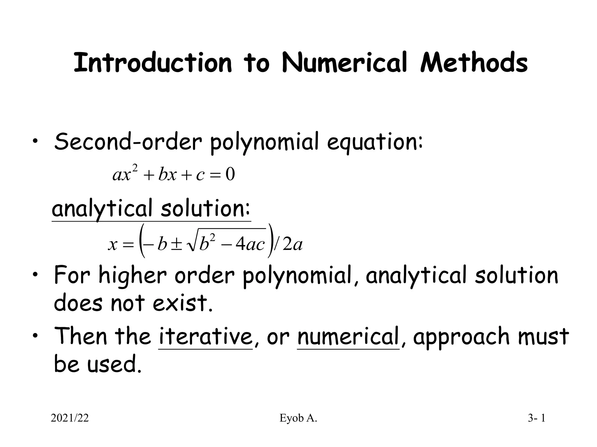
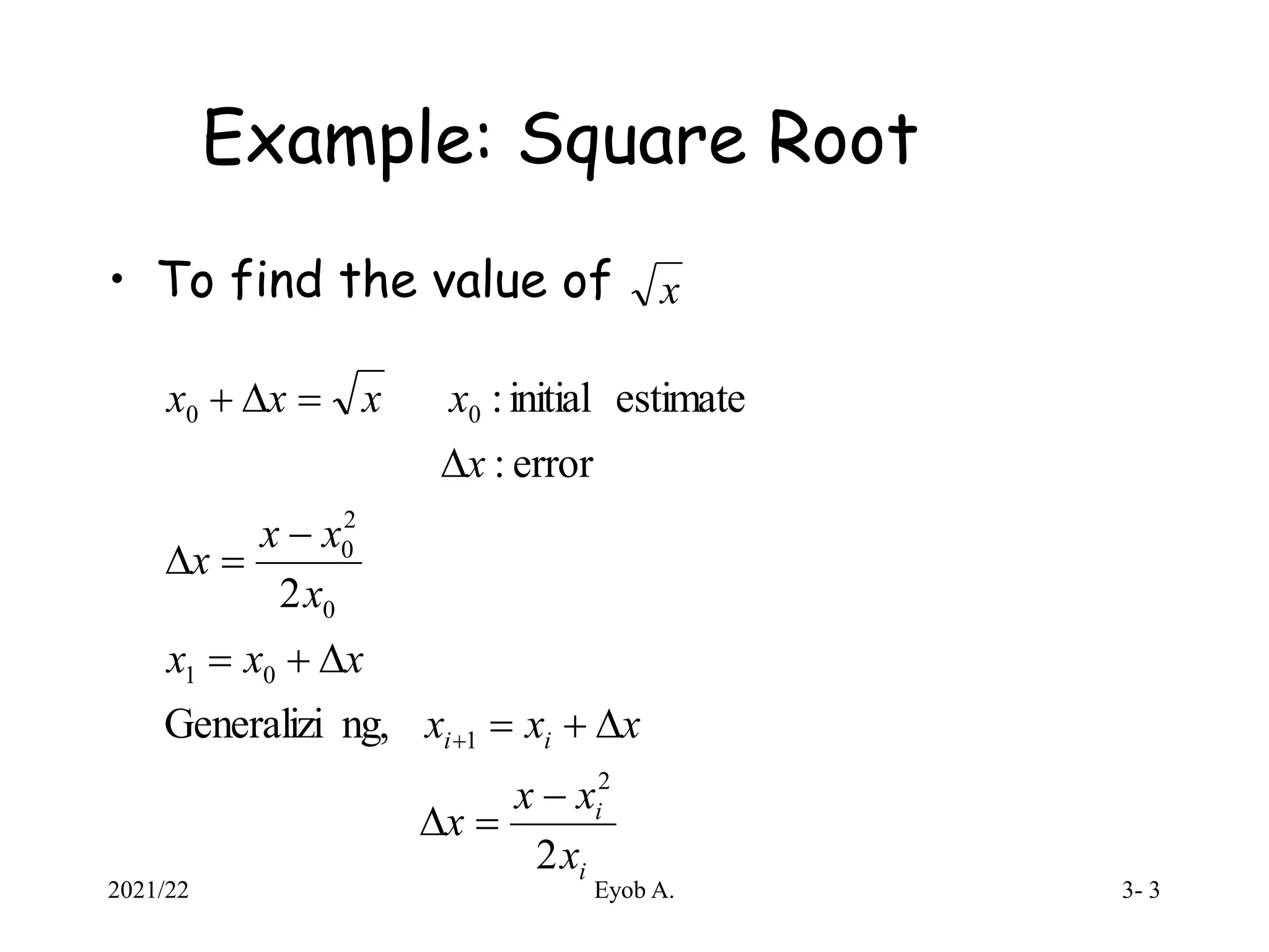
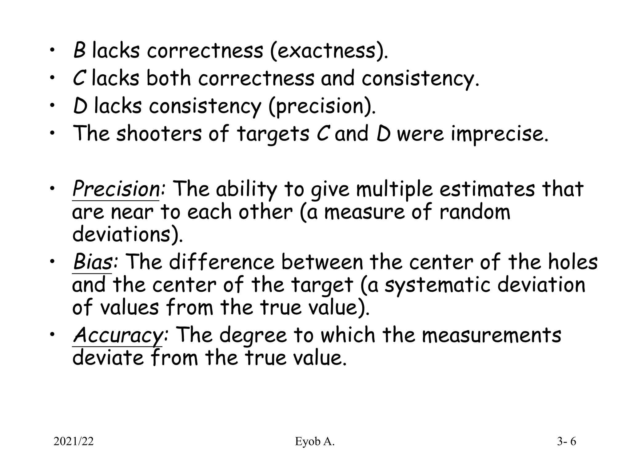
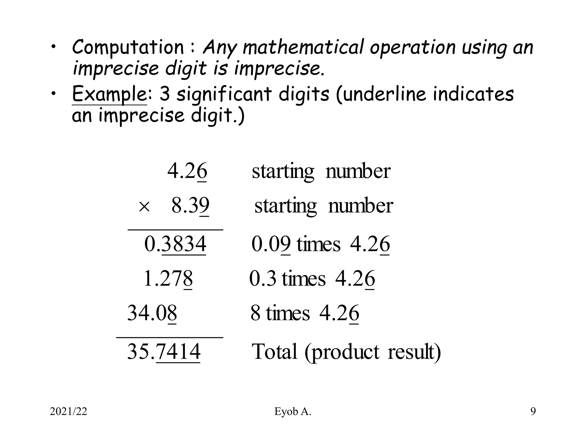
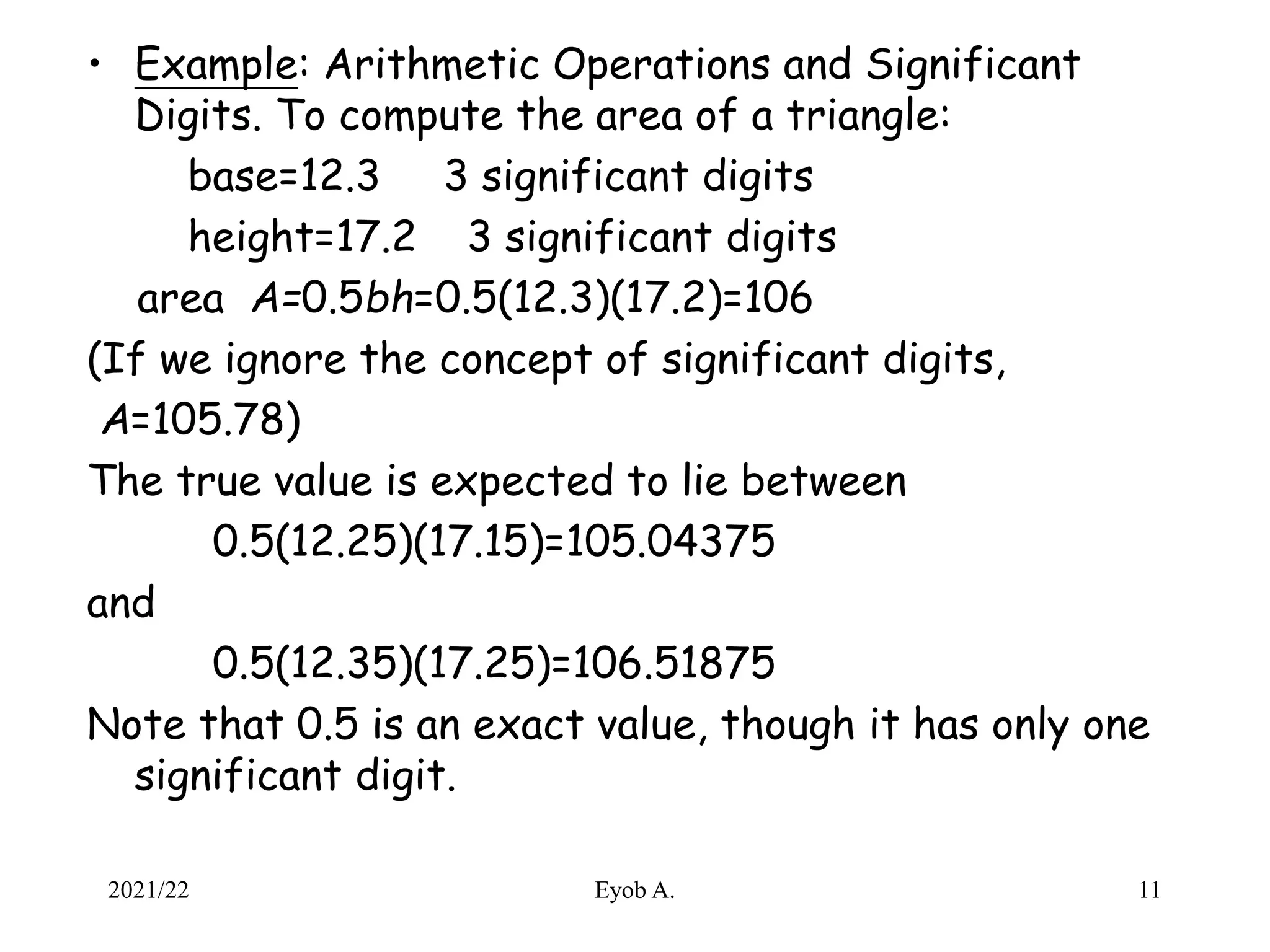
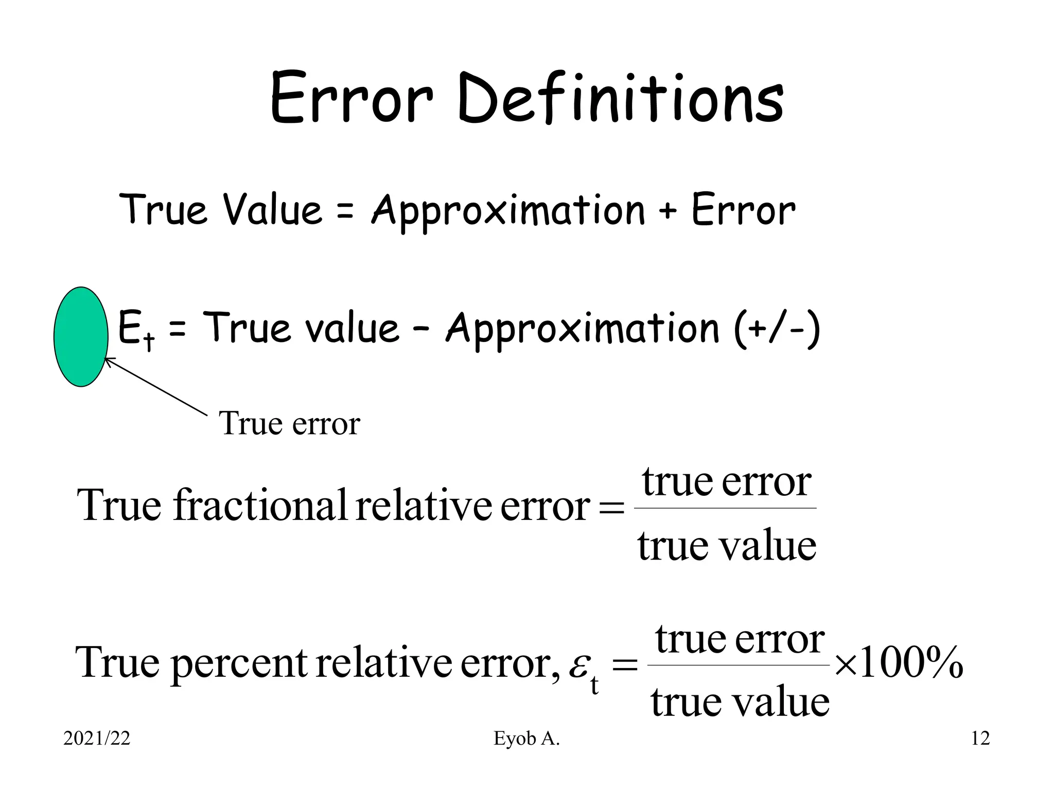
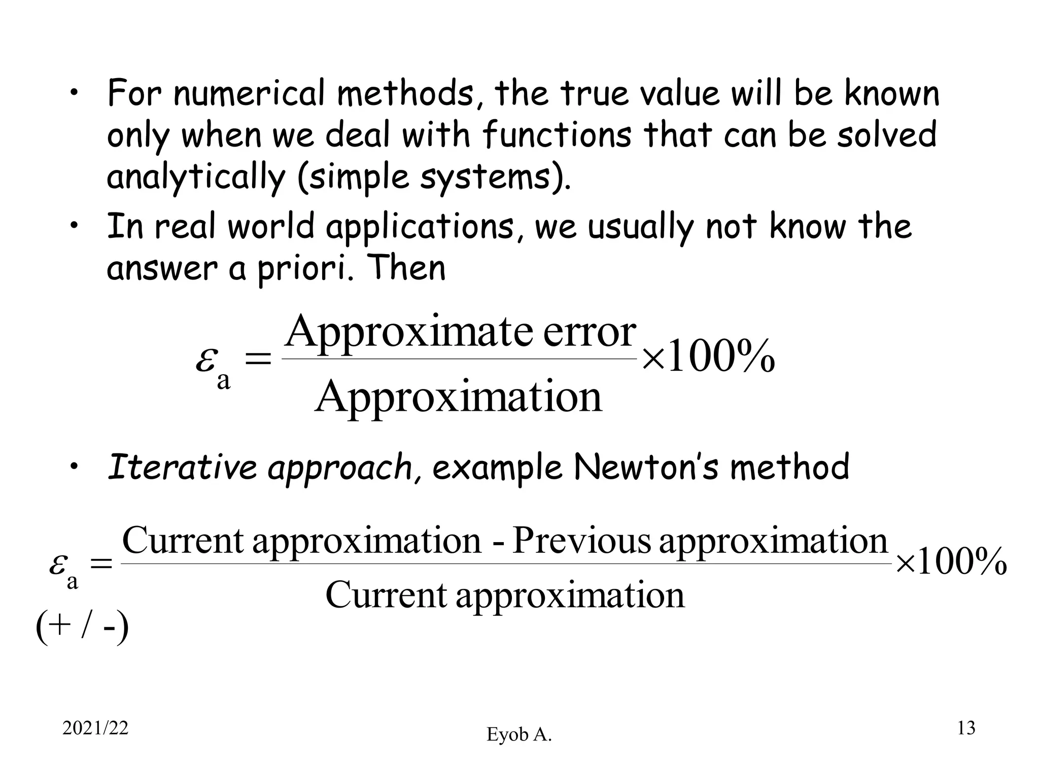
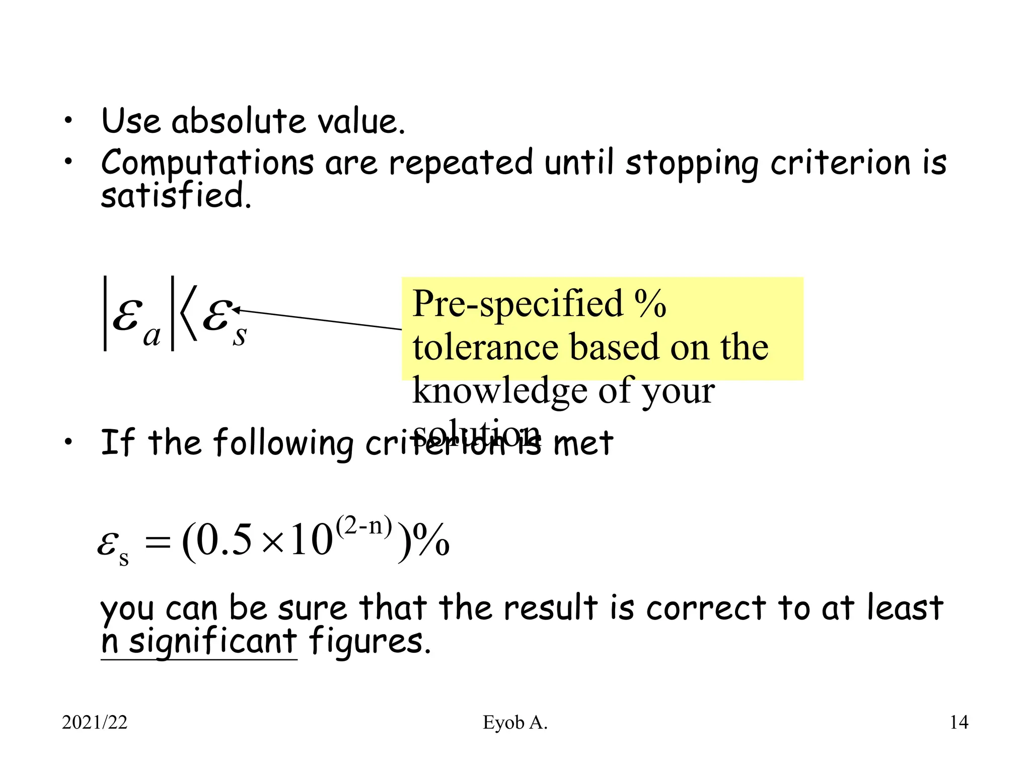
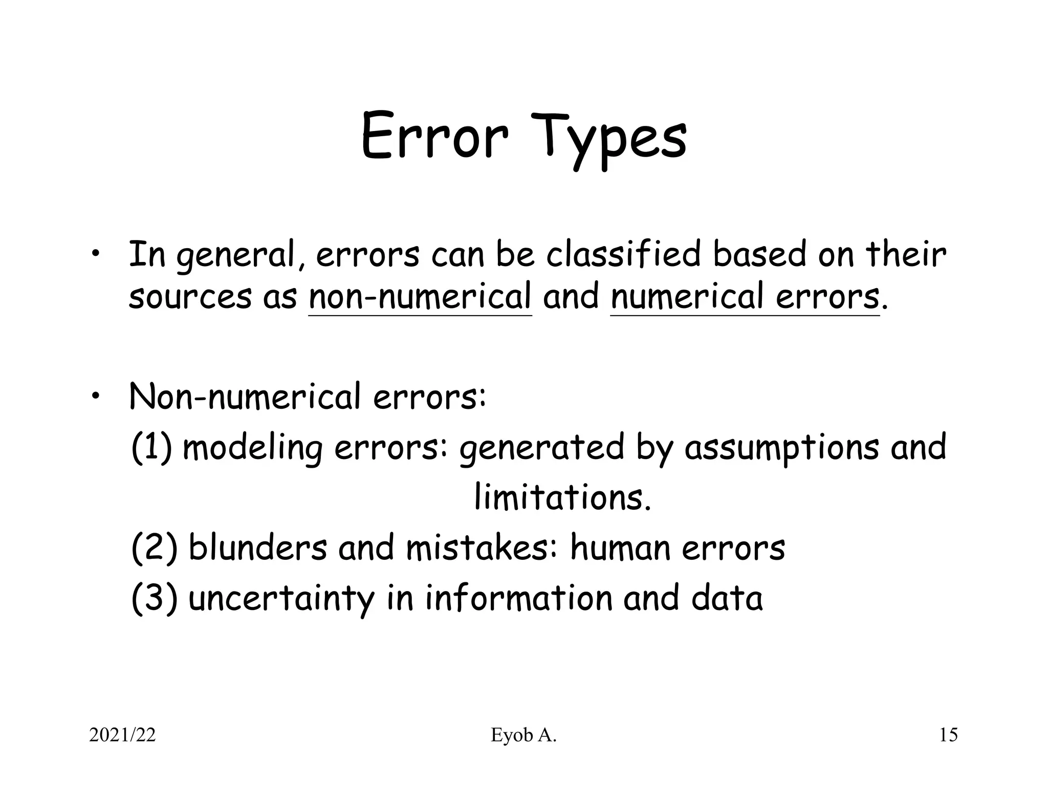
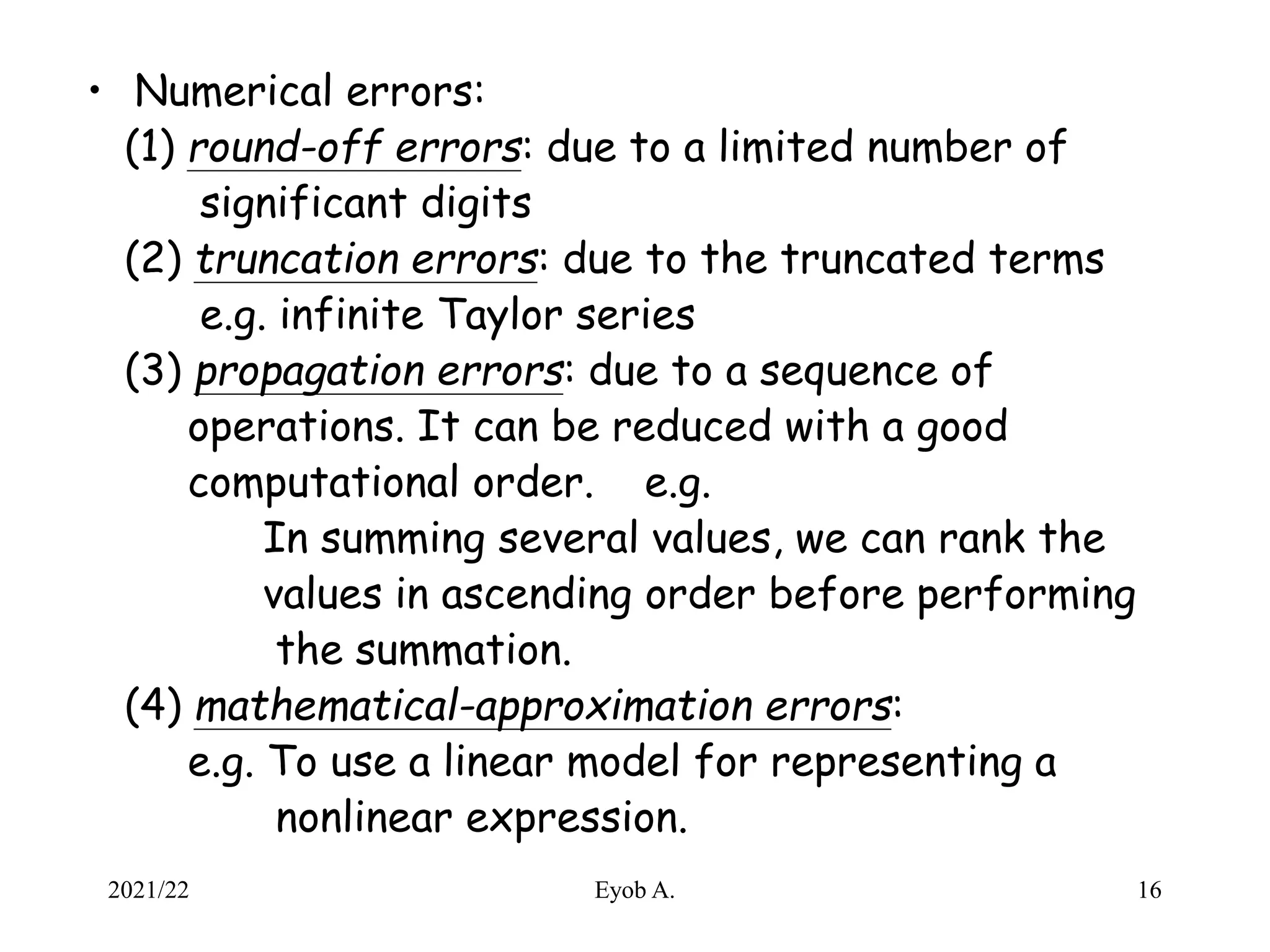
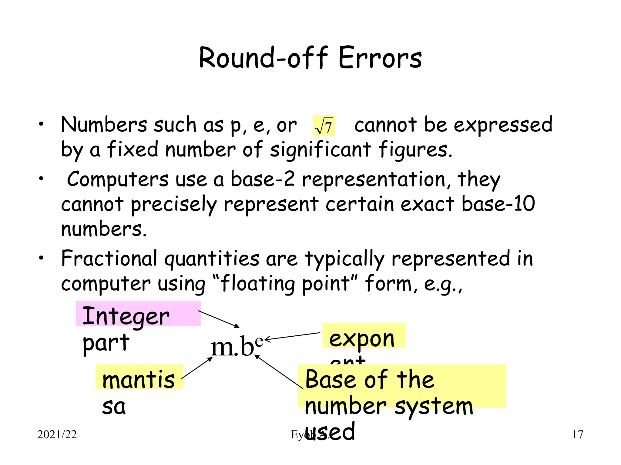
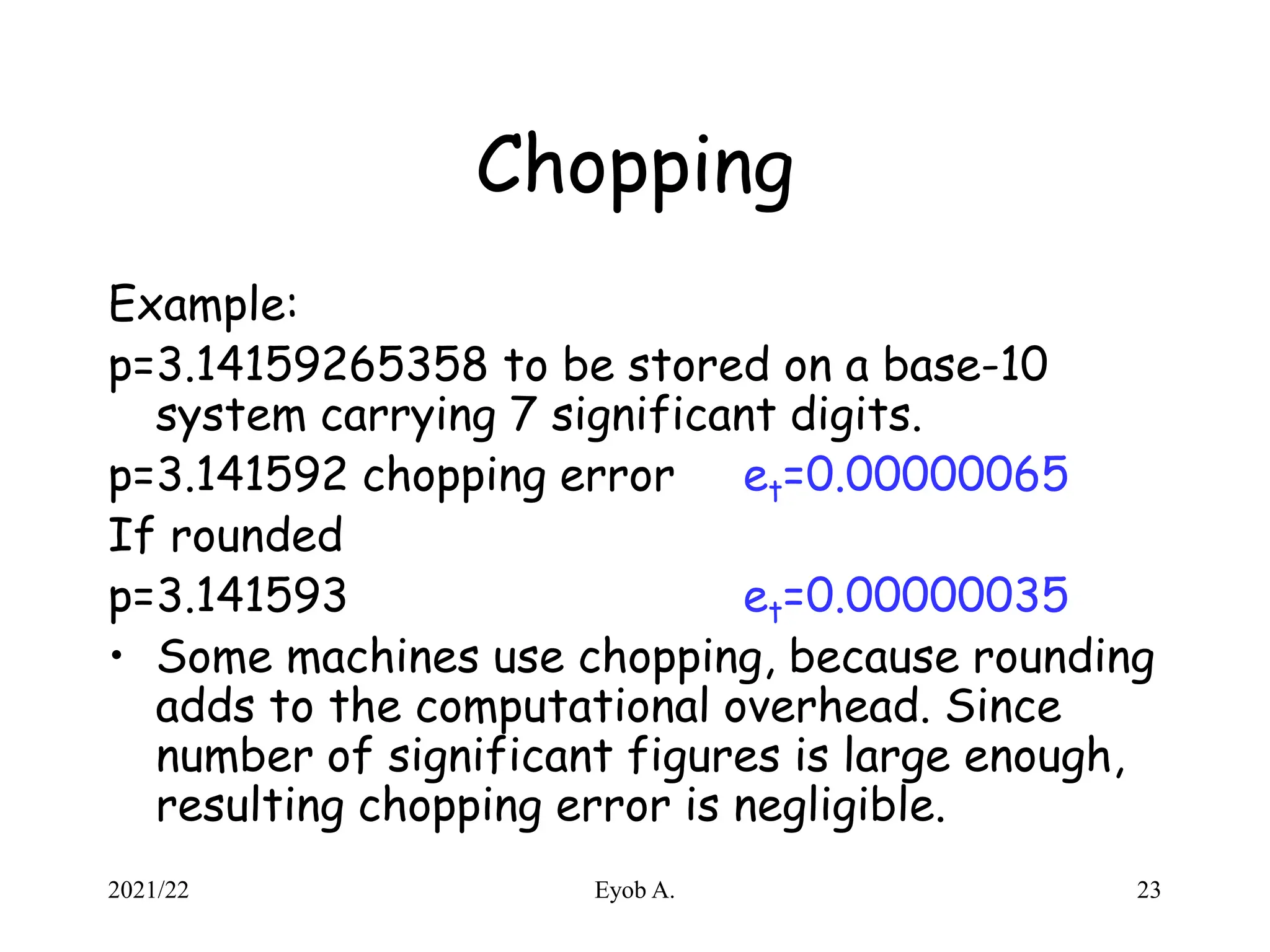
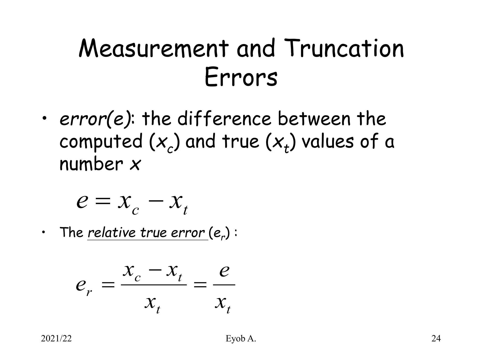
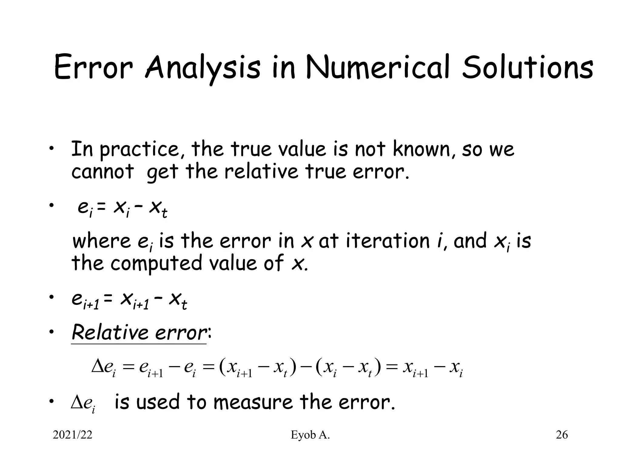
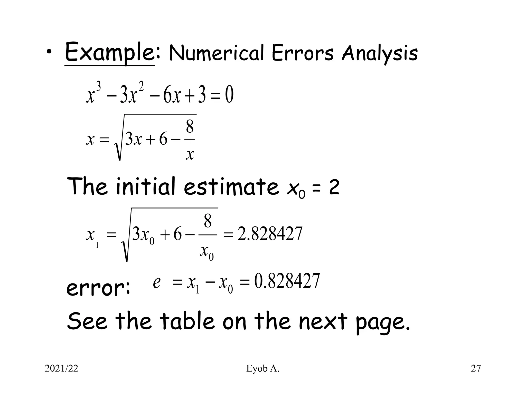
SlideShare a Scribd company logo
1 of 28
Introduction to Numerical Methods
• Second-order polynomial equation:
analytical solution:
• For higher order polynomial, analytical solution
does not exist.
• Then the iterative, or numerical, approach must
be used.
0
2


 c
bx
ax
  a
ac
b
b
x 2
/
4
2




2021/22 Eyob A. 3- 1
Characteristics of Numerical Methods
1. The solution procedure is iterative, with the
accuracy of the solution improving with each
iteration.
2. The solution procedure provides only an
approximation to the true, but unknown, solution.
3. An initial estimate of the solution may be
required.
4. The algorithm is simple and can be easily
programmed.
5. The solution procedure may occasionally diverge
from rather than converge to the true solution.
2021/22 Eyob A. 3- 2
Example: Square Root
• To find the value of x
i
i
i
i
x
x
x
x
x
x
x
x
x
x
x
x
x
x
x
x
x
x
x
2
ng,
Generalizi
2
error
:
estimate
initial
:
2
1
0
1
0
2
0
0
0

















2021/22 Eyob A. 3- 3
• Assume x=150. Because 122=144, let x0=12.
25
.
0
)
12
(
2
12
150
2
2
0
2
0






x
x
x
x
5
2
2
2
2
10
12861
.
0
)
24745
.
12
(
2
)
24745
.
12
(
150
2









x
x
x
x
00255
.
0
)
25
.
12
(
2
)
25
.
12
(
150
2
2
1
2
1







x
x
x
x
24744871
.
12
150
:
solution
true 
2021/22 Eyob A. 3- 4
Accuracy, Precision and Bias
• Four shooting results:
• A is successful.
• B : holes agree with each other (consistency or
precision), but they deviate considerably from
where the shooter was aiming (no correctness)
2021/22 Eyob A. 3- 5
• B lacks correctness (exactness).
• C lacks both correctness and consistency.
• D lacks consistency (precision).
• The shooters of targets C and D were imprecise.
• Precision: The ability to give multiple estimates that
are near to each other (a measure of random
deviations).
• Bias: The difference between the center of the holes
and the center of the target (a systematic deviation
of values from the true value).
• Accuracy: The degree to which the measurements
deviate from the true value.
2021/22 Eyob A. 3- 6
Summary of Bias, Precision and
Accuracy
Target Bias Precision Accuracy
A
None
(unbiased)
High High
B High High Low
C
None
(unbiased)
Low Low
D Moderate Low Low
2021/22 Eyob A. 3- 7
Significant Figures
• The digits from 1 to 9 are always significant.
• Zero being significant where it is not being used
to set the position of the decimal point.
• 2410, 2.41, 0.00241: three significant digits
(0 in 2410 is only used to set the decimal place.)
• Scientific notation can be used to avoid confusion:
2.41×10³: three significant digits
2.410×10³: four significant digits
2021/22 Eyob A. 8
• Computation : Any mathematical operation using an
imprecise digit is imprecise.
• Example: 3 significant digits (underline indicates
an imprecise digit.)
result)
(product
Total
7414
35.
6
4.2
times
8
8
34.0
6
4.2
times
0.3
8
1.27
6
4.2
times
9
0.0
3834
0.
number
starting
9
8.3
number
starting
6
2
.
4

2021/22 Eyob A. 9
x
Y 9860
.
1
587
.
11
ˆ 

digits
t
significan
three
99
.
1
6
.
11
ˆ
3 x
Y 

Table: Rounding Numerical Calculations
1 13.59 13.576 13.573
20 51.40 51.310 51.307
40 91.20 91.030 91.027
100 210.60 210.19 210.187
x 3
ˆ
Y 4
ˆ
Y 5
Ŷ
digits
t
significan
four
986
.
1
59
.
11
ˆ4 x
Y 

digits
t
significan
five
9860
.
1
587
.
11
ˆ
5 x
Y 

• Example: Compute
Rounding should be made at the end of computation,
not at intermediate calculation
2021/22 Eyob A. 10
• Example: Arithmetic Operations and Significant
Digits. To compute the area of a triangle:
base=12.3 3 significant digits
height=17.2 3 significant digits
area A=0.5bh=0.5(12.3)(17.2)=106
(If we ignore the concept of significant digits,
A=105.78)
The true value is expected to lie between
0.5(12.25)(17.15)=105.04375
and
0.5(12.35)(17.25)=106.51875
Note that 0.5 is an exact value, though it has only one
significant digit.
2021/22 Eyob A. 11
Error Definitions
True Value = Approximation + Error
Et = True value – Approximation (+/-)
value
true
error
true
error
relative
fractional
True 
%
100
value
true
error
true
error,
relative
percent
True t



2021/22 Eyob A.
True error
12
• For numerical methods, the true value will be known
only when we deal with functions that can be solved
analytically (simple systems).
• In real world applications, we usually not know the
answer a priori. Then
• Iterative approach, example Newton’s method
%
100
ion
Approximat
error
e
Approximat
a



%
100
ion
approximat
Current
ion
approximat
Previous
-
ion
approximat
Current
a



2021/22 Eyob A.
(+ / -)
13
• Use absolute value.
• Computations are repeated until stopping criterion is
satisfied.
• If the following criterion is met
you can be sure that the result is correct to at least
n significant figures.
s
a 
 
)%
10
(0.5 n)
-
(2
s 


2021/22 Eyob A.
Pre-specified %
tolerance based on the
knowledge of your
solution
14
Error Types
• In general, errors can be classified based on their
sources as non-numerical and numerical errors.
• Non-numerical errors:
(1) modeling errors: generated by assumptions and
limitations.
(2) blunders and mistakes: human errors
(3) uncertainty in information and data
2021/22 Eyob A. 15
• Numerical errors:
(1) round-off errors: due to a limited number of
significant digits
(2) truncation errors: due to the truncated terms
e.g. infinite Taylor series
(3) propagation errors: due to a sequence of
operations. It can be reduced with a good
computational order. e.g.
In summing several values, we can rank the
values in ascending order before performing
the summation.
(4) mathematical-approximation errors:
e.g. To use a linear model for representing a
nonlinear expression.
2021/22 Eyob A. 16
Round-off Errors
• Numbers such as p, e, or cannot be expressed
by a fixed number of significant figures.
• Computers use a base-2 representation, they
cannot precisely represent certain exact base-10
numbers.
• Fractional quantities are typically represented in
computer using “floating point” form, e.g.,
7
e
m.b
2021/22 Eyob A.
expon
ent
Base of the
number system
used
mantis
sa
Integer
part
17
Figure 3.3
2021/22 Eyob A. 18
Figure 3.4
2021/22 Eyob A. 19
2021/22 Eyob A. 20
156.78  0.15678x10³ in a floating
point base-10 system
• Normalized to remove the leading zeroes.
• Multiply the mantissa by 10 and lower the exponent by
1
0.2941 x 10⁻¹
1
2
1
10
0294
.
0
029411765
.
0
34
1
0 



m
2021/22 Eyob A.
Additional significant figure is
retained
Suppose only 4 decimal places
to be stored
21
Therefore
for a base-10 system 0.1 ≤m<1
for a base-2 system 0.5 ≤m<1
• Floating point representation allows both fractions
and very large numbers to be expressed on the
computer. However,
– Floating point numbers take up more room.
– Take longer to process than integer numbers.
– Round-off errors are introduced because mantissa
holds only a finite number of significant figures.
1
1

 m
b
2021/22 Eyob A. 22
Chopping
Example:
p=3.14159265358 to be stored on a base-10
system carrying 7 significant digits.
p=3.141592 chopping error et=0.00000065
If rounded
p=3.141593 et=0.00000035
• Some machines use chopping, because rounding
adds to the computational overhead. Since
number of significant figures is large enough,
resulting chopping error is negligible.
2021/22 Eyob A. 23
Measurement and Truncation
Errors
• error(e): the difference between the
computed (xc) and true (xt) values of a
number x
• The relative true error (er) :
t
c x
x
e 

t
t
t
c
r
x
e
x
x
x
e 


2021/22 Eyob A. 24
• Example: Truncation Error in Atomic Weight
The weight of oxygen is 15.9994.
If we round the atomic weight of oxygen to 16,
the error is
e = 16 - 15.9994 - 0.0006
The relative true error:
4
10
4
.
0
9994
.
15
0006
.
0 



r
e
2021/22 Eyob A. 25
Error Analysis in Numerical Solutions
• In practice, the true value is not known, so we
cannot get the relative true error.
• ei = xi – xt
where ei is the error in x at iteration i, and xi is
the computed value of x.
• ei+1 = xi+1 – xt
• Relative error:
• is used to measure the error.
i
i
t
i
t
i
i
i
i x
x
x
x
x
x
e
e
e 







 

 1
1
1 )
(
)
(
i
e

2021/22 Eyob A. 26
• Example: Numerical Errors Analysis
The initial estimate x0 = 2
error:
See the table on the next page.
0
3
6
3 2
3



 x
x
x
x
x
x
8
6
3 


828427
.
2
8
6
3
0
0
1




x
x
x
828427
.
0
0
1 

 x
x
e
2021/22 Eyob A. 27
Table: Error Analysis with xt =4
Trail
0 2.000000 - 2.000000
1 2.828427 0.828427 1.171573
2 3.414214 0.582786 0.585786
3 3.728203 0.313989 0.271797
4 3.877989 0.149787 0.122011
5 3.946016 0.068027 0.053984
6 3.976265 0.030249 0.023735
7 3.989594 0.013328 0.010406
8 3.995443 0.005849 0.004557
9 3.998005
0000256
3
0.001995
i
x i
e
 i
t x
x 
i
2021/22 Eyob A. 28

More Related Content

Similar to Chapter 1 Errors and Approximations.ppt

C language numanal
C language numanalC language numanal
C language numanalaluavi
 
Course Name: Digital System Design Number System.pdf
Course Name: Digital System Design Number System.pdfCourse Name: Digital System Design Number System.pdf
Course Name: Digital System Design Number System.pdfMdJubayerFaisalEmon
 
data representation
 data representation data representation
data representationHaroon_007
 
Chapter 2.1 introduction to number system
Chapter 2.1 introduction to number systemChapter 2.1 introduction to number system
Chapter 2.1 introduction to number systemISMT College
 
Unit One - Solved problems on error analysis .ppt
Unit One - Solved problems on error analysis .pptUnit One - Solved problems on error analysis .ppt
Unit One - Solved problems on error analysis .pptashugizaw1506
 
A floating-point adder (IEEE 754 floating-point.pptx
A floating-point adder (IEEE 754 floating-point.pptxA floating-point adder (IEEE 754 floating-point.pptx
A floating-point adder (IEEE 754 floating-point.pptxNiveditaAcharyya2035
 
Logic Circuits Design - "Chapter 1: Digital Systems and Information"
Logic Circuits Design - "Chapter 1: Digital Systems and Information"Logic Circuits Design - "Chapter 1: Digital Systems and Information"
Logic Circuits Design - "Chapter 1: Digital Systems and Information"Ra'Fat Al-Msie'deen
 
Only floating point lecture 7 (1)
Only floating point lecture 7 (1)Only floating point lecture 7 (1)
Only floating point lecture 7 (1)talhashahid40
 
Finite word length effects
Finite word length effectsFinite word length effects
Finite word length effectsPeriyanayagiS
 
12 13 h2_measurement_ppt
12 13 h2_measurement_ppt12 13 h2_measurement_ppt
12 13 h2_measurement_pptTan Hong
 

Similar to Chapter 1 Errors and Approximations.ppt (20)

Numerical Method
Numerical Method Numerical Method
Numerical Method
 
C language numanal
C language numanalC language numanal
C language numanal
 
Course Name: Digital System Design Number System.pdf
Course Name: Digital System Design Number System.pdfCourse Name: Digital System Design Number System.pdf
Course Name: Digital System Design Number System.pdf
 
data representation
 data representation data representation
data representation
 
Cse115 lecture01numbersystems
Cse115 lecture01numbersystemsCse115 lecture01numbersystems
Cse115 lecture01numbersystems
 
Chapter 2.1 introduction to number system
Chapter 2.1 introduction to number systemChapter 2.1 introduction to number system
Chapter 2.1 introduction to number system
 
Unit One - Solved problems on error analysis .ppt
Unit One - Solved problems on error analysis .pptUnit One - Solved problems on error analysis .ppt
Unit One - Solved problems on error analysis .ppt
 
A floating-point adder (IEEE 754 floating-point.pptx
A floating-point adder (IEEE 754 floating-point.pptxA floating-point adder (IEEE 754 floating-point.pptx
A floating-point adder (IEEE 754 floating-point.pptx
 
Informe #1 de metodos
Informe #1 de metodosInforme #1 de metodos
Informe #1 de metodos
 
1
11
1
 
Logic Circuits Design - "Chapter 1: Digital Systems and Information"
Logic Circuits Design - "Chapter 1: Digital Systems and Information"Logic Circuits Design - "Chapter 1: Digital Systems and Information"
Logic Circuits Design - "Chapter 1: Digital Systems and Information"
 
Alu1
Alu1Alu1
Alu1
 
Digital Logic
Digital LogicDigital Logic
Digital Logic
 
Only floating point lecture 7 (1)
Only floating point lecture 7 (1)Only floating point lecture 7 (1)
Only floating point lecture 7 (1)
 
Lecture 2 ns
Lecture 2 nsLecture 2 ns
Lecture 2 ns
 
Simplex Algorithm
Simplex AlgorithmSimplex Algorithm
Simplex Algorithm
 
Finite word length effects
Finite word length effectsFinite word length effects
Finite word length effects
 
12 13 h2_measurement_ppt
12 13 h2_measurement_ppt12 13 h2_measurement_ppt
12 13 h2_measurement_ppt
 
Number system
Number systemNumber system
Number system
 
ITC lecture 3.pptx
ITC lecture 3.pptxITC lecture 3.pptx
ITC lecture 3.pptx
 

Recently uploaded

SOCIAL AND HISTORICAL CONTEXT - LFTVD.pptx
SOCIAL AND HISTORICAL CONTEXT - LFTVD.pptxSOCIAL AND HISTORICAL CONTEXT - LFTVD.pptx
SOCIAL AND HISTORICAL CONTEXT - LFTVD.pptxiammrhaywood
 
Mastering the Unannounced Regulatory Inspection
Mastering the Unannounced Regulatory InspectionMastering the Unannounced Regulatory Inspection
Mastering the Unannounced Regulatory InspectionSafetyChain Software
 
Presentation by Andreas Schleicher Tackling the School Absenteeism Crisis 30 ...
Presentation by Andreas Schleicher Tackling the School Absenteeism Crisis 30 ...Presentation by Andreas Schleicher Tackling the School Absenteeism Crisis 30 ...
Presentation by Andreas Schleicher Tackling the School Absenteeism Crisis 30 ...EduSkills OECD
 
Industrial Policy - 1948, 1956, 1973, 1977, 1980, 1991
Industrial Policy - 1948, 1956, 1973, 1977, 1980, 1991Industrial Policy - 1948, 1956, 1973, 1977, 1980, 1991
Industrial Policy - 1948, 1956, 1973, 1977, 1980, 1991RKavithamani
 
Organic Name Reactions for the students and aspirants of Chemistry12th.pptx
Organic Name Reactions  for the students and aspirants of Chemistry12th.pptxOrganic Name Reactions  for the students and aspirants of Chemistry12th.pptx
Organic Name Reactions for the students and aspirants of Chemistry12th.pptxVS Mahajan Coaching Centre
 
microwave assisted reaction. General introduction
microwave assisted reaction. General introductionmicrowave assisted reaction. General introduction
microwave assisted reaction. General introductionMaksud Ahmed
 
Sanyam Choudhary Chemistry practical.pdf
Sanyam Choudhary Chemistry practical.pdfSanyam Choudhary Chemistry practical.pdf
Sanyam Choudhary Chemistry practical.pdfsanyamsingh5019
 
Crayon Activity Handout For the Crayon A
Crayon Activity Handout For the Crayon ACrayon Activity Handout For the Crayon A
Crayon Activity Handout For the Crayon AUnboundStockton
 
Arihant handbook biology for class 11 .pdf
Arihant handbook biology for class 11 .pdfArihant handbook biology for class 11 .pdf
Arihant handbook biology for class 11 .pdfchloefrazer622
 
Concept of Vouching. B.Com(Hons) /B.Compdf
Concept of Vouching. B.Com(Hons) /B.CompdfConcept of Vouching. B.Com(Hons) /B.Compdf
Concept of Vouching. B.Com(Hons) /B.CompdfUmakantAnnand
 
Alper Gobel In Media Res Media Component
Alper Gobel In Media Res Media ComponentAlper Gobel In Media Res Media Component
Alper Gobel In Media Res Media ComponentInMediaRes1
 
Q4-W6-Restating Informational Text Grade 3
Q4-W6-Restating Informational Text Grade 3Q4-W6-Restating Informational Text Grade 3
Q4-W6-Restating Informational Text Grade 3JemimahLaneBuaron
 
18-04-UA_REPORT_MEDIALITERAСY_INDEX-DM_23-1-final-eng.pdf
18-04-UA_REPORT_MEDIALITERAСY_INDEX-DM_23-1-final-eng.pdf18-04-UA_REPORT_MEDIALITERAСY_INDEX-DM_23-1-final-eng.pdf
18-04-UA_REPORT_MEDIALITERAСY_INDEX-DM_23-1-final-eng.pdfssuser54595a
 
Solving Puzzles Benefits Everyone (English).pptx
Solving Puzzles Benefits Everyone (English).pptxSolving Puzzles Benefits Everyone (English).pptx
Solving Puzzles Benefits Everyone (English).pptxOH TEIK BIN
 
mini mental status format.docx
mini    mental       status     format.docxmini    mental       status     format.docx
mini mental status format.docxPoojaSen20
 
PSYCHIATRIC History collection FORMAT.pptx
PSYCHIATRIC   History collection FORMAT.pptxPSYCHIATRIC   History collection FORMAT.pptx
PSYCHIATRIC History collection FORMAT.pptxPoojaSen20
 

Recently uploaded (20)

SOCIAL AND HISTORICAL CONTEXT - LFTVD.pptx
SOCIAL AND HISTORICAL CONTEXT - LFTVD.pptxSOCIAL AND HISTORICAL CONTEXT - LFTVD.pptx
SOCIAL AND HISTORICAL CONTEXT - LFTVD.pptx
 
Mastering the Unannounced Regulatory Inspection
Mastering the Unannounced Regulatory InspectionMastering the Unannounced Regulatory Inspection
Mastering the Unannounced Regulatory Inspection
 
Presentation by Andreas Schleicher Tackling the School Absenteeism Crisis 30 ...
Presentation by Andreas Schleicher Tackling the School Absenteeism Crisis 30 ...Presentation by Andreas Schleicher Tackling the School Absenteeism Crisis 30 ...
Presentation by Andreas Schleicher Tackling the School Absenteeism Crisis 30 ...
 
Industrial Policy - 1948, 1956, 1973, 1977, 1980, 1991
Industrial Policy - 1948, 1956, 1973, 1977, 1980, 1991Industrial Policy - 1948, 1956, 1973, 1977, 1980, 1991
Industrial Policy - 1948, 1956, 1973, 1977, 1980, 1991
 
Organic Name Reactions for the students and aspirants of Chemistry12th.pptx
Organic Name Reactions  for the students and aspirants of Chemistry12th.pptxOrganic Name Reactions  for the students and aspirants of Chemistry12th.pptx
Organic Name Reactions for the students and aspirants of Chemistry12th.pptx
 
microwave assisted reaction. General introduction
microwave assisted reaction. General introductionmicrowave assisted reaction. General introduction
microwave assisted reaction. General introduction
 
Sanyam Choudhary Chemistry practical.pdf
Sanyam Choudhary Chemistry practical.pdfSanyam Choudhary Chemistry practical.pdf
Sanyam Choudhary Chemistry practical.pdf
 
TataKelola dan KamSiber Kecerdasan Buatan v022.pdf
TataKelola dan KamSiber Kecerdasan Buatan v022.pdfTataKelola dan KamSiber Kecerdasan Buatan v022.pdf
TataKelola dan KamSiber Kecerdasan Buatan v022.pdf
 
Crayon Activity Handout For the Crayon A
Crayon Activity Handout For the Crayon ACrayon Activity Handout For the Crayon A
Crayon Activity Handout For the Crayon A
 
Arihant handbook biology for class 11 .pdf
Arihant handbook biology for class 11 .pdfArihant handbook biology for class 11 .pdf
Arihant handbook biology for class 11 .pdf
 
Concept of Vouching. B.Com(Hons) /B.Compdf
Concept of Vouching. B.Com(Hons) /B.CompdfConcept of Vouching. B.Com(Hons) /B.Compdf
Concept of Vouching. B.Com(Hons) /B.Compdf
 
Model Call Girl in Bikash Puri Delhi reach out to us at 🔝9953056974🔝
Model Call Girl in Bikash Puri  Delhi reach out to us at 🔝9953056974🔝Model Call Girl in Bikash Puri  Delhi reach out to us at 🔝9953056974🔝
Model Call Girl in Bikash Puri Delhi reach out to us at 🔝9953056974🔝
 
Alper Gobel In Media Res Media Component
Alper Gobel In Media Res Media ComponentAlper Gobel In Media Res Media Component
Alper Gobel In Media Res Media Component
 
Q4-W6-Restating Informational Text Grade 3
Q4-W6-Restating Informational Text Grade 3Q4-W6-Restating Informational Text Grade 3
Q4-W6-Restating Informational Text Grade 3
 
Código Creativo y Arte de Software | Unidad 1
Código Creativo y Arte de Software | Unidad 1Código Creativo y Arte de Software | Unidad 1
Código Creativo y Arte de Software | Unidad 1
 
Staff of Color (SOC) Retention Efforts DDSD
Staff of Color (SOC) Retention Efforts DDSDStaff of Color (SOC) Retention Efforts DDSD
Staff of Color (SOC) Retention Efforts DDSD
 
18-04-UA_REPORT_MEDIALITERAСY_INDEX-DM_23-1-final-eng.pdf
18-04-UA_REPORT_MEDIALITERAСY_INDEX-DM_23-1-final-eng.pdf18-04-UA_REPORT_MEDIALITERAСY_INDEX-DM_23-1-final-eng.pdf
18-04-UA_REPORT_MEDIALITERAСY_INDEX-DM_23-1-final-eng.pdf
 
Solving Puzzles Benefits Everyone (English).pptx
Solving Puzzles Benefits Everyone (English).pptxSolving Puzzles Benefits Everyone (English).pptx
Solving Puzzles Benefits Everyone (English).pptx
 
mini mental status format.docx
mini    mental       status     format.docxmini    mental       status     format.docx
mini mental status format.docx
 
PSYCHIATRIC History collection FORMAT.pptx
PSYCHIATRIC   History collection FORMAT.pptxPSYCHIATRIC   History collection FORMAT.pptx
PSYCHIATRIC History collection FORMAT.pptx
 

Chapter 1 Errors and Approximations.ppt

  • 1. Introduction to Numerical Methods • Second-order polynomial equation: analytical solution: • For higher order polynomial, analytical solution does not exist. • Then the iterative, or numerical, approach must be used. 0 2    c bx ax   a ac b b x 2 / 4 2     2021/22 Eyob A. 3- 1
  • 2. Characteristics of Numerical Methods 1. The solution procedure is iterative, with the accuracy of the solution improving with each iteration. 2. The solution procedure provides only an approximation to the true, but unknown, solution. 3. An initial estimate of the solution may be required. 4. The algorithm is simple and can be easily programmed. 5. The solution procedure may occasionally diverge from rather than converge to the true solution. 2021/22 Eyob A. 3- 2
  • 3. Example: Square Root • To find the value of x i i i i x x x x x x x x x x x x x x x x x x x 2 ng, Generalizi 2 error : estimate initial : 2 1 0 1 0 2 0 0 0                  2021/22 Eyob A. 3- 3
  • 4. • Assume x=150. Because 122=144, let x0=12. 25 . 0 ) 12 ( 2 12 150 2 2 0 2 0       x x x x 5 2 2 2 2 10 12861 . 0 ) 24745 . 12 ( 2 ) 24745 . 12 ( 150 2          x x x x 00255 . 0 ) 25 . 12 ( 2 ) 25 . 12 ( 150 2 2 1 2 1        x x x x 24744871 . 12 150 : solution true  2021/22 Eyob A. 3- 4
  • 5. Accuracy, Precision and Bias • Four shooting results: • A is successful. • B : holes agree with each other (consistency or precision), but they deviate considerably from where the shooter was aiming (no correctness) 2021/22 Eyob A. 3- 5
  • 6. • B lacks correctness (exactness). • C lacks both correctness and consistency. • D lacks consistency (precision). • The shooters of targets C and D were imprecise. • Precision: The ability to give multiple estimates that are near to each other (a measure of random deviations). • Bias: The difference between the center of the holes and the center of the target (a systematic deviation of values from the true value). • Accuracy: The degree to which the measurements deviate from the true value. 2021/22 Eyob A. 3- 6
  • 7. Summary of Bias, Precision and Accuracy Target Bias Precision Accuracy A None (unbiased) High High B High High Low C None (unbiased) Low Low D Moderate Low Low 2021/22 Eyob A. 3- 7
  • 8. Significant Figures • The digits from 1 to 9 are always significant. • Zero being significant where it is not being used to set the position of the decimal point. • 2410, 2.41, 0.00241: three significant digits (0 in 2410 is only used to set the decimal place.) • Scientific notation can be used to avoid confusion: 2.41×10³: three significant digits 2.410×10³: four significant digits 2021/22 Eyob A. 8
  • 9. • Computation : Any mathematical operation using an imprecise digit is imprecise. • Example: 3 significant digits (underline indicates an imprecise digit.) result) (product Total 7414 35. 6 4.2 times 8 8 34.0 6 4.2 times 0.3 8 1.27 6 4.2 times 9 0.0 3834 0. number starting 9 8.3 number starting 6 2 . 4  2021/22 Eyob A. 9
  • 10. x Y 9860 . 1 587 . 11 ˆ   digits t significan three 99 . 1 6 . 11 ˆ 3 x Y   Table: Rounding Numerical Calculations 1 13.59 13.576 13.573 20 51.40 51.310 51.307 40 91.20 91.030 91.027 100 210.60 210.19 210.187 x 3 ˆ Y 4 ˆ Y 5 Ŷ digits t significan four 986 . 1 59 . 11 ˆ4 x Y   digits t significan five 9860 . 1 587 . 11 ˆ 5 x Y   • Example: Compute Rounding should be made at the end of computation, not at intermediate calculation 2021/22 Eyob A. 10
  • 11. • Example: Arithmetic Operations and Significant Digits. To compute the area of a triangle: base=12.3 3 significant digits height=17.2 3 significant digits area A=0.5bh=0.5(12.3)(17.2)=106 (If we ignore the concept of significant digits, A=105.78) The true value is expected to lie between 0.5(12.25)(17.15)=105.04375 and 0.5(12.35)(17.25)=106.51875 Note that 0.5 is an exact value, though it has only one significant digit. 2021/22 Eyob A. 11
  • 12. Error Definitions True Value = Approximation + Error Et = True value – Approximation (+/-) value true error true error relative fractional True  % 100 value true error true error, relative percent True t    2021/22 Eyob A. True error 12
  • 13. • For numerical methods, the true value will be known only when we deal with functions that can be solved analytically (simple systems). • In real world applications, we usually not know the answer a priori. Then • Iterative approach, example Newton’s method % 100 ion Approximat error e Approximat a    % 100 ion approximat Current ion approximat Previous - ion approximat Current a    2021/22 Eyob A. (+ / -) 13
  • 14. • Use absolute value. • Computations are repeated until stopping criterion is satisfied. • If the following criterion is met you can be sure that the result is correct to at least n significant figures. s a    )% 10 (0.5 n) - (2 s    2021/22 Eyob A. Pre-specified % tolerance based on the knowledge of your solution 14
  • 15. Error Types • In general, errors can be classified based on their sources as non-numerical and numerical errors. • Non-numerical errors: (1) modeling errors: generated by assumptions and limitations. (2) blunders and mistakes: human errors (3) uncertainty in information and data 2021/22 Eyob A. 15
  • 16. • Numerical errors: (1) round-off errors: due to a limited number of significant digits (2) truncation errors: due to the truncated terms e.g. infinite Taylor series (3) propagation errors: due to a sequence of operations. It can be reduced with a good computational order. e.g. In summing several values, we can rank the values in ascending order before performing the summation. (4) mathematical-approximation errors: e.g. To use a linear model for representing a nonlinear expression. 2021/22 Eyob A. 16
  • 17. Round-off Errors • Numbers such as p, e, or cannot be expressed by a fixed number of significant figures. • Computers use a base-2 representation, they cannot precisely represent certain exact base-10 numbers. • Fractional quantities are typically represented in computer using “floating point” form, e.g., 7 e m.b 2021/22 Eyob A. expon ent Base of the number system used mantis sa Integer part 17
  • 21. 156.78  0.15678x10³ in a floating point base-10 system • Normalized to remove the leading zeroes. • Multiply the mantissa by 10 and lower the exponent by 1 0.2941 x 10⁻¹ 1 2 1 10 0294 . 0 029411765 . 0 34 1 0     m 2021/22 Eyob A. Additional significant figure is retained Suppose only 4 decimal places to be stored 21
  • 22. Therefore for a base-10 system 0.1 ≤m<1 for a base-2 system 0.5 ≤m<1 • Floating point representation allows both fractions and very large numbers to be expressed on the computer. However, – Floating point numbers take up more room. – Take longer to process than integer numbers. – Round-off errors are introduced because mantissa holds only a finite number of significant figures. 1 1   m b 2021/22 Eyob A. 22
  • 23. Chopping Example: p=3.14159265358 to be stored on a base-10 system carrying 7 significant digits. p=3.141592 chopping error et=0.00000065 If rounded p=3.141593 et=0.00000035 • Some machines use chopping, because rounding adds to the computational overhead. Since number of significant figures is large enough, resulting chopping error is negligible. 2021/22 Eyob A. 23
  • 24. Measurement and Truncation Errors • error(e): the difference between the computed (xc) and true (xt) values of a number x • The relative true error (er) : t c x x e   t t t c r x e x x x e    2021/22 Eyob A. 24
  • 25. • Example: Truncation Error in Atomic Weight The weight of oxygen is 15.9994. If we round the atomic weight of oxygen to 16, the error is e = 16 - 15.9994 - 0.0006 The relative true error: 4 10 4 . 0 9994 . 15 0006 . 0     r e 2021/22 Eyob A. 25
  • 26. Error Analysis in Numerical Solutions • In practice, the true value is not known, so we cannot get the relative true error. • ei = xi – xt where ei is the error in x at iteration i, and xi is the computed value of x. • ei+1 = xi+1 – xt • Relative error: • is used to measure the error. i i t i t i i i i x x x x x x e e e             1 1 1 ) ( ) ( i e  2021/22 Eyob A. 26
  • 27. • Example: Numerical Errors Analysis The initial estimate x0 = 2 error: See the table on the next page. 0 3 6 3 2 3     x x x x x x 8 6 3    828427 . 2 8 6 3 0 0 1     x x x 828427 . 0 0 1    x x e 2021/22 Eyob A. 27
  • 28. Table: Error Analysis with xt =4 Trail 0 2.000000 - 2.000000 1 2.828427 0.828427 1.171573 2 3.414214 0.582786 0.585786 3 3.728203 0.313989 0.271797 4 3.877989 0.149787 0.122011 5 3.946016 0.068027 0.053984 6 3.976265 0.030249 0.023735 7 3.989594 0.013328 0.010406 8 3.995443 0.005849 0.004557 9 3.998005 0000256 3 0.001995 i x i e  i t x x  i 2021/22 Eyob A. 28