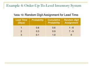
Downloaded 3,577 times
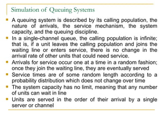
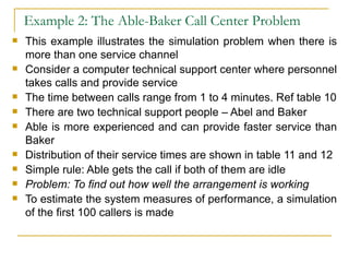
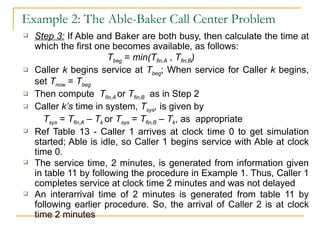
![Simulation of Queuing Systems Service just completed flow diagram No Yes If unit has just completed service, simulation proceeds as above: [Departure event occurs when unit completes service] Server has only two possible states – busy or idle Departure event Another unit waiting? Begin Server idle time Remove waiting unit from queue Begin servicing the unit](https://image.slidesharecdn.com/chp-2simulationexamples-110202104329-phpapp02/85/Chp-2-simulation-examples-6-320.jpg)
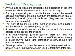
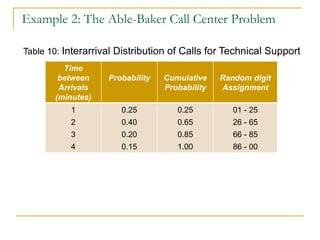
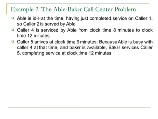
![Simulation of Queuing Systems Unit entering system flow diagram No Yes If unit has just entered the system, simulation proceeds as above: [Arrival event occurs when unit enters system] Unit will find server either busy/idle; unit begins service immediately or enters queue for server It is not possible for server to be idle while queue is nonempty Arrival event Server Busy? Unit enters service Unit enters queue for service](https://image.slidesharecdn.com/chp-2simulationexamples-110202104329-phpapp02/85/Chp-2-simulation-examples-7-320.jpg)
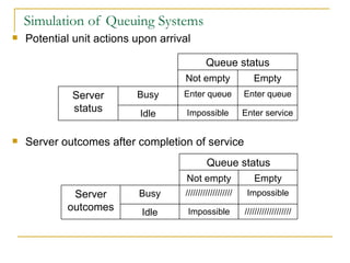
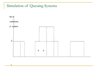
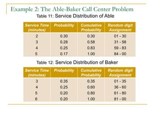
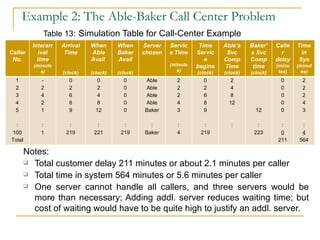
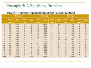
![Example 1: Single-Channel Queue Some of the findings from the simulation table 9 are: [All time figures are in minutes] Average waiting time = total time customers wait in queue = 174 = 1.74 total number of customers 100 Probability that customer has to wait in queue = number of customers who wait = 46 = 0.46 total number of customers 100 Proportion of idle time of server = total idle time of server = 101 = 0.24 total run time of simulation 418 Average service time = total service time = 317 = 3.17 total no. of customers 100 [ compare to expected service time given by equation E(s) = Σ sp(s), s = 0 to ∞ = 1(0.1) + 2(0.2) + 3(0.3) + 4(0.25) + 5(0.1) + 6(0.05) = 3.2 ]](https://image.slidesharecdn.com/chp-2simulationexamples-110202104329-phpapp02/85/Chp-2-simulation-examples-25-320.jpg)
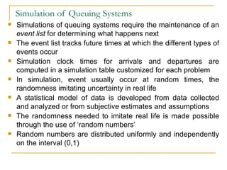
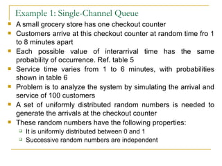
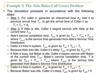
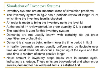
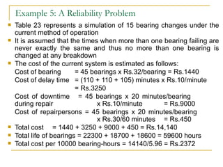
![Example 1: Single-Channel Queue Some of the findings from the simulation table 9 are: Average time between arrivals = sum of all times between arrivals number of arrivals - 1 = 415 / 99 = 4.19 [ compare the above time with expected time between arrivals by finding mean of discrete uniform distribution whose endpoints are a = 1 & b = 8 Mean E(A) = (a + b) / 2 = (1 + 8)/2 = 4.5 ] Average waiting time of = total time customers wait in queue those who wait total number of customers that wait = 174 / 54 = 3.22 Average time customer = total time customers spend in system spends in system total number of customers = 491 / 100 = 4.91 [ another way to find the same is to add average time customers spends waiting in queue and average time customers spends in service = 1.74 + 3.17 = 4.91 ]](https://image.slidesharecdn.com/chp-2simulationexamples-110202104329-phpapp02/85/Chp-2-simulation-examples-26-320.jpg)

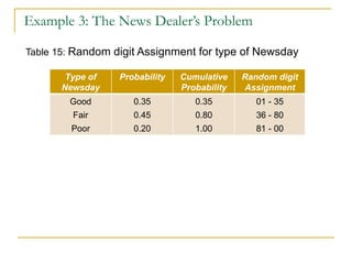

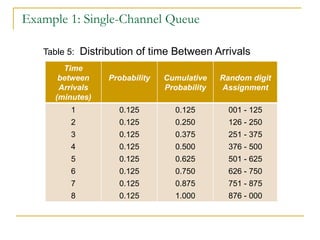
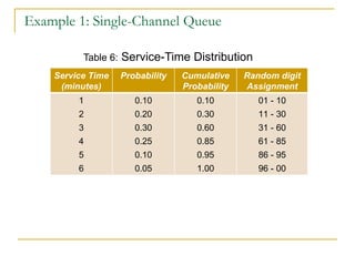
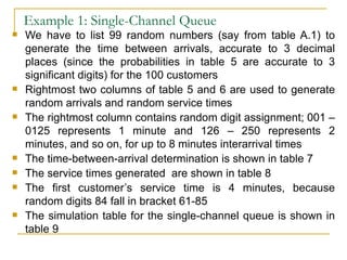
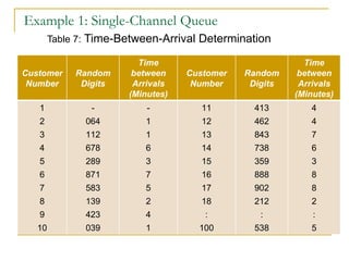
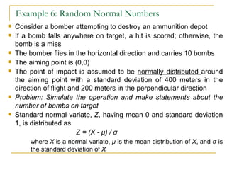
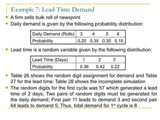
![Example 3: The News Dealer’s Problem The profit for 20-day period is the sum of daily profits, Rs.131.00 Also computed from total for 20 days of simulation Total profit = 600 - 462 + 17 - 10 = Rs.131.00 [462 = cost of newspaper = 20 x 0.33 x 70]](https://image.slidesharecdn.com/chp-2simulationexamples-110202104329-phpapp02/85/Chp-2-simulation-examples-45-320.jpg)
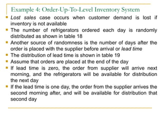
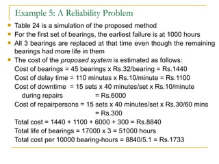
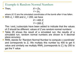
![Table 20: Simulation Table for [M,N] Inventory System Day Cycle Day within Cycle Beginning Inventory Random Digits for Demand Demand Ending Inventory Shortage Quantity Order Quantity Random Digits for Demand Lead Time (days) Days until Order Arrives 1 2 3 4 5 6 7 8 9 10 11 12 13 14 15 16 17 18 19 20 21 22 23 24 25 Total 1 1 1 1 1 2 2 2 2 2 3 3 3 3 3 4 4 4 4 4 5 5 5 5 5 1 2 3 4 5 1 2 3 4 5 1 2 3 4 5 1 2 3 4 5 1 2 3 4 5 3 2 8 7 5 2 1 9 5 3 0 0 11 6 3 2 11 7 5 2 0 12 8 4 3 26 68 33 39 86 18 64 79 55 74 21 43 49 90 35 08 98 61 85 81 53 15 94 19 44 1 2 1 2 3 1 2 3 2 3 1 2 2 3 1 0 4 2 3 3 2 1 4 1 2 2 0 7 5 2 1 0 5 3 0 0 0 6 3 2 2 7 5 2 0 0 8 4 3 1 68 0 0 0 0 0 0 1 0 0 0 1 3 0 0 0 0 0 0 0 1 3 0 0 0 0 9 - - - - 9 - - - - 11 - - - - 9 - - - - 12 - - - - 10 - - - - 8 - - - - 7 - - - - 2 - - - - 3 - - - - 1 - - - - 2 - - - - 2 - - - - 1 - - - - 1 - - - - 1 1 - - - 2 1 - - - 2 1 - - - 1 - - - - 1 - - - - 1](https://image.slidesharecdn.com/chp-2simulationexamples-110202104329-phpapp02/85/Chp-2-simulation-examples-52-320.jpg)
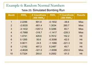
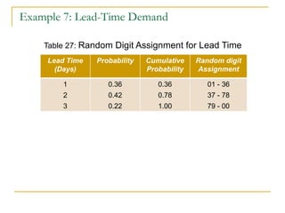
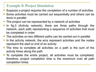

![Example 8: Project Simulation The time that the project (breakfast of eggs, toast and bacon) will be completed is the maximum time through any of the paths But since activities are assumed to be some random variability, the time through the paths are not constant For a uniform distribution, a simulated activity is given by [Pritsker]: Simulated Activity Time = Lower limit + (Upper limit - Lower limit) * Random number The time for each simulated activity can be computed as follows: Example: for activity Start -> A, if random number is 0.7943, the simulated activity time is 2 + (4 - 2) * 0.7943 = 3.59 minutes Simulate using Experiment worksheet (downloaded from www.bcnn.net ) in the Excel workbook for this example and compute the average, median, minimum and maximum values. With 400 trials using default seed, results were as follows: Mean 10.12, Min 6.85, and Max 12.00 minutes](https://image.slidesharecdn.com/chp-2simulationexamples-110202104329-phpapp02/85/Chp-2-simulation-examples-72-320.jpg)
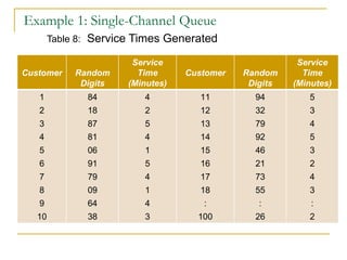
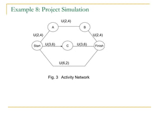
![Example 8: Project Simulation The time that the project (breakfast of eggs, toast and bacon) will be completed is the maximum time through any of the paths But since activities are assumed to be some random variability, the time through the paths are not constant For a uniform distribution, a simulated activity is given by [Pritsker]: Simulated Activity Time = Lower limit + (Upper limit - Lower limit) * Random number The time for each simulated activity can be computed as follows: Example: for activity Start -> A, if random number is 0.7943, the simulated activity time is 2 + (4 - 2) * 0.7943 = 3.59 minutes Simulate using Experiment worksheet (downloaded from www.bcnn.net ) in the Excel workbook for this example and compute the average, median, minimum and maximum values. With 400 trials using default seed, results were as follows: Mean 10.12, Min 6.85, and Max 12.00 minutes](https://image.slidesharecdn.com/chp-2simulationexamples-110202104329-phpapp02/85/Chp-2-simulation-examples-73-320.jpg)
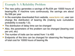
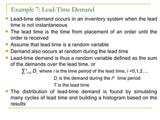
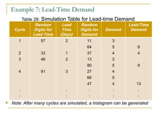
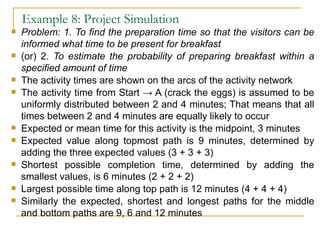
![Example 8: Project Simulation The critical path is the path that takes the longest time for completion; that is, its time is the project completion time For each of the 400 trials, the experiment determines at which path was critical, with these results: Top path 30.00% of trials Middle path 31.25% Bottom path 38.75% Conclusion is that the chance of the bacon being the last item ready is 38.75%. [Question: Why aren’t the paths each represented about 1/3 of the time?] The project completion times were placed in a frequency chart; These differ each time that spreadsheet is recalculated, but, in any large number of trials, the basic shape of the chart (or histogram) will remain roughly the same; Inferences drawn from fig. is that: 13.5% of time (54/400), breakfast will be ready in <=9 minutes 20.5% of time (82/400), it will take 11 to 12 minutes](https://image.slidesharecdn.com/chp-2simulationexamples-110202104329-phpapp02/85/Chp-2-simulation-examples-74-320.jpg)

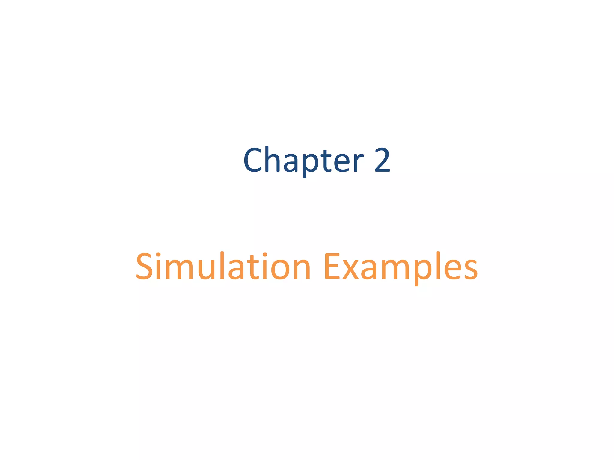
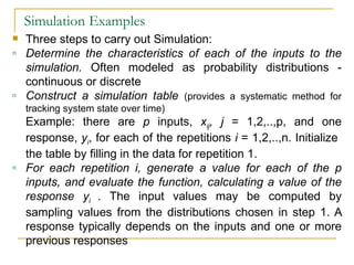
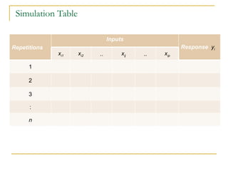
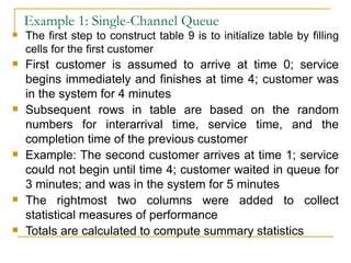
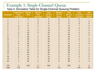
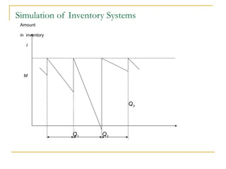
This document discusses simulation examples and simulation of queuing systems. It provides three key steps to carry out a simulation: 1) determine input characteristics, 2) construct a simulation table to track the system state over time, and 3) initialize and run the simulation. It then gives an example of simulating a single-channel queue, including generating random interarrival and service times from distributions and constructing a simulation table. Key performance measures like average wait time and server idle time are calculated from the table.


![System simulation & modeling notes[sjbit]](https://cdn.slidesharecdn.com/ss_thumbnails/systemsimulationmodelingnotessjbit-110929031610-phpapp01-thumbnail.jpg?width=640&height=640&fit=bounds)