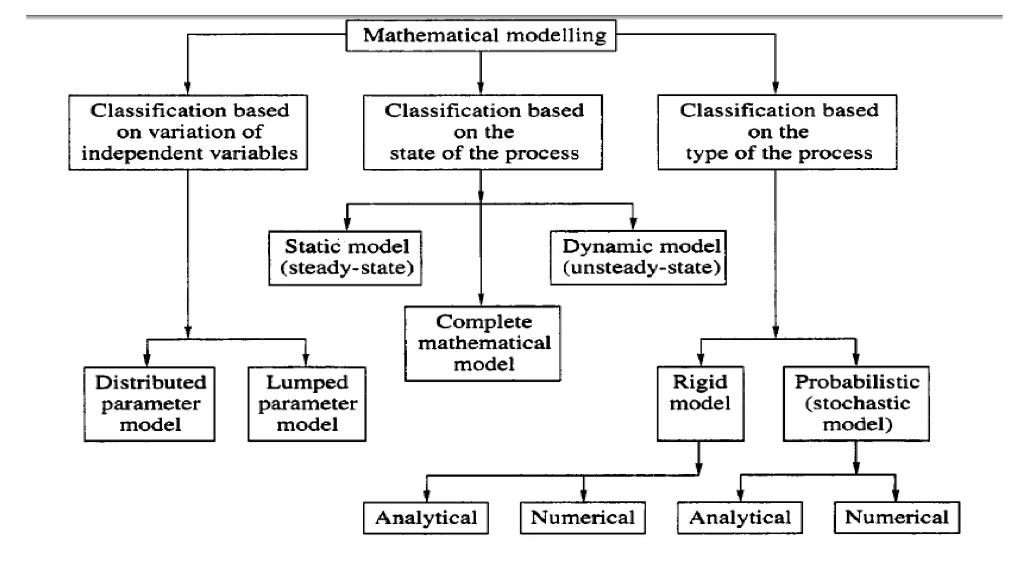
TYPES OF MODELS
&
METHAMATICAL
MODELING
PROCESS MODELING, SIMULATION & OPTIMIZATION
Classification of mathematical modeling
• Independent variables These are quantities describing a system that can be
varied by choice during a particular experiment, independent of one another.
Examples include time and coordinate variables.
• Dependent variables These are the properties of a system which change when
the independent variables are altered in value. There is no direct control over a
dependent variable during an experiment. The relationship between independent
and dependent variables is one of cause and efect; independent variables
measure the cause and dependent variables measure the eflect. Examples for
dependent variables include temperature, concentration and efficiency.
Classification based on Variation of
Independent Variables
• This classification of mathematical modelling is done based on whether the process
variables vary with time as an independent variable or with both time and space coordinates
as independent variables.
Distributed Parameter Models
• If the basic process variables vary with both time and space, or if these changes occur
only with space of dimension exceeding unity (i.e., more than one space coordinate), such
processes are represented by distributed parameter (DP) models, which are formulated as
partial differential equations.
Lumped Parameter Models
• Processes in which the basic process variables vary only with time are represented by
lumped parameter (LP) models, which are formulated as ordinary differential equations.
Classification Based on the State of the Process
• The primary objective of cybernetics is to control a given system or process.
As a consequence, a complete mathematical model is expected to describe
relationships between the basic process variables under steady-state conditions
(a static model) and transient conditions (a dynamic model).
Static Model
• A static or steady-state model ignores the changes in process variables with
time. The construction of a static model involves the following steps:
Step 1 Analysis of the process to establish its physical and chemical nature, its
objective, the governing equations describing a given class of processes and also
its specific features as a unit process.
Step 2 Identification and ascertaining of the input and output variables of the
process. The variables include (see Fig. 3.3) the following:
2. Manipulated variables: Variables that directly affect the course of the process
Static Model
3. Disturbances: Variables that directly affect the course of the process but C Y
j). and that can be measured and changed purposefully (xi). that cannot be
changed purposefully (q).
4. Intermediate variables: Variables related to the course of the process only
indirectly (xni).
• Step 3 Identification and establishing of the relationships, constraints, and
boundary conditions of the process. The static model of a unit process should
allow for all possible modes of operation of the typical reactor.
Dynamic Model
• The construction of a dynamic or unsteady-state model reduces to obtaining the
dynamic characteristics of the process, i.e., establishing relationships between its main
variables as they change with time.
• Dynamic characteristics can be obtained by theory, experiment, or both. In obtaining
dynamic characteristics experimentally, disturbances are applied to the input of a
system and the time response to the disturbance is noted. Such experiments are based on
the laws of signal flow dealt with in information arid control theory. The dynamic
model of a process may take the form of any of the following:
1. A set of transfer functions relating the selected dependent variable to one
2. Ordinary or partial differential equations derived theoretically and
3. Equations derived for the various elements of the unit process that may be or several
independent variables. containing all the necessary dependent and independent
variables. analyzed independently of one another.
Classification Based on the Type of the
Process
• Depending on whether a given process is deterministic or stochastic, it
may be represented by any one of the following mathematical models:
1. An analytical rigid model
2. A numerical rigid model
3. An analytical probabilistic model
4. A numerical probabilistic model
• It may be noted that in some practical cases a model cannot be classified
under any of the above headings. The choice of a particular type of model
is to a great extent determined by the simplicity of the solution it offers.
Rigid or Deterministic Models
• These models usually describe deterministic processes without the use of
probability distributions. As mentioned above, the subclassification of rigid (or
deterministic) models is analytical rigid models and numerical rigid models,
depending on whether the solution is obtained analytically or numerically. This
is not to say that the underlying phenomena, especially when a numerical rigid
model is used, are not statistical in character. This implies that only the averages
and not the whole distributions are dealt with here.
Stochastic or Probabilistic Models
• These models usually represent stochastic (random) processes. Here again, the
sub classification of probabilistic models is analytical probabilistic (or
stochastic) and numerical probabilistic (or stochastic) models, depending on
whether the solution is obtained analytically or numerically. It may be noted
that simulation corresponding to a numerical stochastic model is known as
Monte Car10 simulation.
Comparison Between Rigid and Stochastic
Models
• In constructing rigid models, we use different classical techniques of mathematics,
namely, differential equations, integral equations, linear difference equations, and operators
for conversion to algebraic models and so on. Probabilistic models represent the distribution
of discrete and continuous variables and also sample distributions.
• A major advantage of statistical models (probabilistic) over analytical (rigid) ones is that
these do not call for rough approximations and allow for a greater number of factors. But
these models are difficult to analyse and grasp. From this point of view, it may be preferable
to use less precise analytical models. The best results are obtained when both analytical and
statistical models are used jointly in conjunction with each other. A simple analytical model
will give an insight into the basic behaviour of the prototype system and suggest further
approaches in which statistical models of any complexity can be used. Residence time
distribution (RTD) models are good examples of this approach.

Types of models

  • 1.
    TYPES OF MODELS & METHAMATICAL MODELING PROCESSMODELING, SIMULATION & OPTIMIZATION
  • 2.
    Classification of mathematicalmodeling • Independent variables These are quantities describing a system that can be varied by choice during a particular experiment, independent of one another. Examples include time and coordinate variables. • Dependent variables These are the properties of a system which change when the independent variables are altered in value. There is no direct control over a dependent variable during an experiment. The relationship between independent and dependent variables is one of cause and efect; independent variables measure the cause and dependent variables measure the eflect. Examples for dependent variables include temperature, concentration and efficiency.
  • 4.
    Classification based onVariation of Independent Variables • This classification of mathematical modelling is done based on whether the process variables vary with time as an independent variable or with both time and space coordinates as independent variables. Distributed Parameter Models • If the basic process variables vary with both time and space, or if these changes occur only with space of dimension exceeding unity (i.e., more than one space coordinate), such processes are represented by distributed parameter (DP) models, which are formulated as partial differential equations. Lumped Parameter Models • Processes in which the basic process variables vary only with time are represented by lumped parameter (LP) models, which are formulated as ordinary differential equations.
  • 5.
    Classification Based onthe State of the Process • The primary objective of cybernetics is to control a given system or process. As a consequence, a complete mathematical model is expected to describe relationships between the basic process variables under steady-state conditions (a static model) and transient conditions (a dynamic model).
  • 6.
    Static Model • Astatic or steady-state model ignores the changes in process variables with time. The construction of a static model involves the following steps: Step 1 Analysis of the process to establish its physical and chemical nature, its objective, the governing equations describing a given class of processes and also its specific features as a unit process. Step 2 Identification and ascertaining of the input and output variables of the process. The variables include (see Fig. 3.3) the following: 2. Manipulated variables: Variables that directly affect the course of the process
  • 7.
    Static Model 3. Disturbances:Variables that directly affect the course of the process but C Y j). and that can be measured and changed purposefully (xi). that cannot be changed purposefully (q). 4. Intermediate variables: Variables related to the course of the process only indirectly (xni). • Step 3 Identification and establishing of the relationships, constraints, and boundary conditions of the process. The static model of a unit process should allow for all possible modes of operation of the typical reactor.
  • 8.
    Dynamic Model • Theconstruction of a dynamic or unsteady-state model reduces to obtaining the dynamic characteristics of the process, i.e., establishing relationships between its main variables as they change with time. • Dynamic characteristics can be obtained by theory, experiment, or both. In obtaining dynamic characteristics experimentally, disturbances are applied to the input of a system and the time response to the disturbance is noted. Such experiments are based on the laws of signal flow dealt with in information arid control theory. The dynamic model of a process may take the form of any of the following: 1. A set of transfer functions relating the selected dependent variable to one 2. Ordinary or partial differential equations derived theoretically and 3. Equations derived for the various elements of the unit process that may be or several independent variables. containing all the necessary dependent and independent variables. analyzed independently of one another.
  • 9.
    Classification Based onthe Type of the Process • Depending on whether a given process is deterministic or stochastic, it may be represented by any one of the following mathematical models: 1. An analytical rigid model 2. A numerical rigid model 3. An analytical probabilistic model 4. A numerical probabilistic model • It may be noted that in some practical cases a model cannot be classified under any of the above headings. The choice of a particular type of model is to a great extent determined by the simplicity of the solution it offers.
  • 10.
    Rigid or DeterministicModels • These models usually describe deterministic processes without the use of probability distributions. As mentioned above, the subclassification of rigid (or deterministic) models is analytical rigid models and numerical rigid models, depending on whether the solution is obtained analytically or numerically. This is not to say that the underlying phenomena, especially when a numerical rigid model is used, are not statistical in character. This implies that only the averages and not the whole distributions are dealt with here.
  • 11.
    Stochastic or ProbabilisticModels • These models usually represent stochastic (random) processes. Here again, the sub classification of probabilistic models is analytical probabilistic (or stochastic) and numerical probabilistic (or stochastic) models, depending on whether the solution is obtained analytically or numerically. It may be noted that simulation corresponding to a numerical stochastic model is known as Monte Car10 simulation.
  • 12.
    Comparison Between Rigidand Stochastic Models • In constructing rigid models, we use different classical techniques of mathematics, namely, differential equations, integral equations, linear difference equations, and operators for conversion to algebraic models and so on. Probabilistic models represent the distribution of discrete and continuous variables and also sample distributions. • A major advantage of statistical models (probabilistic) over analytical (rigid) ones is that these do not call for rough approximations and allow for a greater number of factors. But these models are difficult to analyse and grasp. From this point of view, it may be preferable to use less precise analytical models. The best results are obtained when both analytical and statistical models are used jointly in conjunction with each other. A simple analytical model will give an insight into the basic behaviour of the prototype system and suggest further approaches in which statistical models of any complexity can be used. Residence time distribution (RTD) models are good examples of this approach.