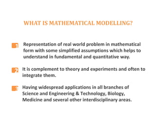
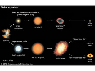
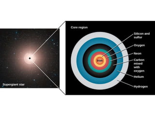
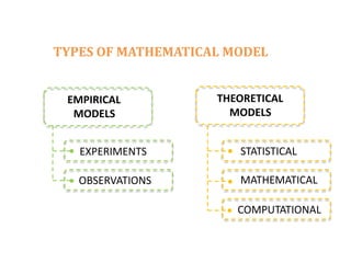
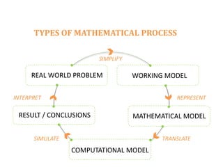
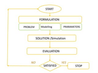
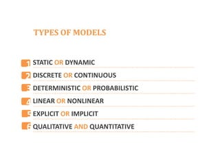
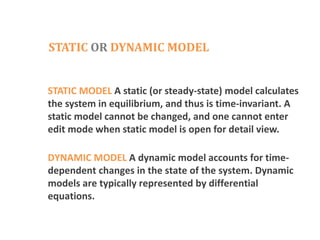
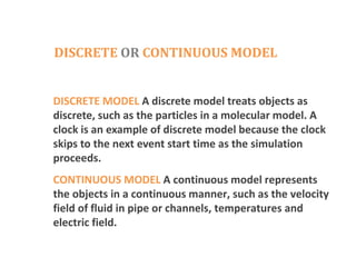
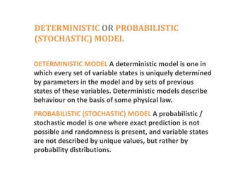
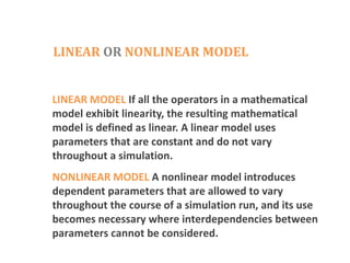
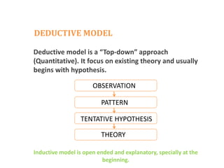
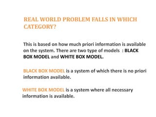
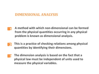
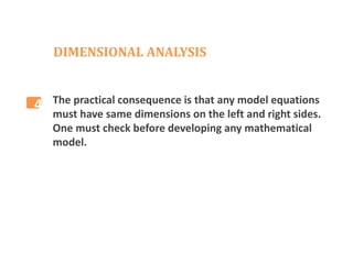
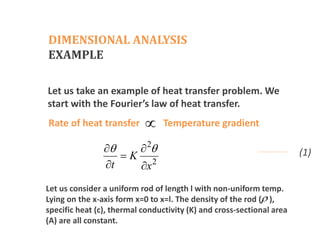
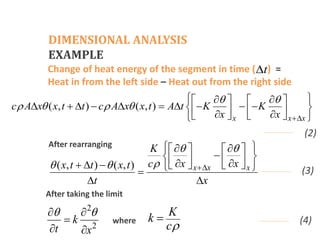
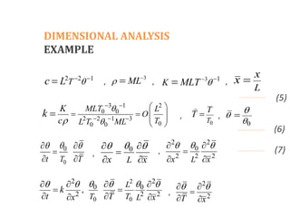
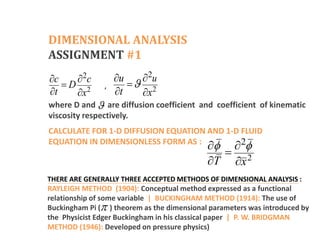
INTRODUCTION TO MATHEMATICAL
MODELLING
Mudassar Ahmed
Education:
● B.Sc. Physics & Double Mathematics (Punjab University, Lahore)
● M.Sc. Physics (University of Gujrat )
● Bachelors in Education: Information and Computer Technology
(Virtual University of Pakistan)
● M.phil (Continued): Astronomy & Astrophysics (Institute of Space
Technology, Islamabad)
Work Experience:
● Physics Teacher in IMSB (Ex-FG Schools & Colleges), Islamabad
● Ex-Lecturer at Aspire Group of Colleges Dina
● Web Developer at SARL Lab
OUTLINES OF THE PRESENTATION
DIMENSIONAL ANALYSIS
WHAT IS MATHEMATICAL MODELLING?
WHY MATHEMATICAL MODEL IS NECESSARY?
USE OF MATHEMATICAL MODEL
TYPES OF MATHEMATICAL MODEL
MATHEMATICAL MODELLING PROCESS
WHAT IS MATHEMATICAL MODELLING?
Representation of real world problem in mathematical
form with some simplified assumptions which helps to
understand in fundamental and quantitative way.
It is complement to theory and experiments and often to
integrate them.
Having widespread applications in all branches of
Science and Engineering & Technology, Biology,
Medicine and several other interdisciplinary areas.
2
3
1
WHY MATHEMATICAL MODEL IS
NECESSARY?
To perform experiments and to solve real world
problems which may be risky and expensive or time
consuming or impossible like astrophysics.
Emerged as a powerful, indispensable tool for studying a
variety of problems in scientific research, product and
process development and manufacturing.
Improves the quality of work and reduced changes,
errors and rework
However, mathematical model is only a complement but does not
replace theory and experimentation in scientific research.
1
2
3
USE OF MATHEMATICAL MODEL
Solves the real world problems and has become wide
spread due to increasing computation power and
computing methods.
Facilitated to handle large scale and complicated
problems.
Some areas where mathematical models are highly used
are : Climate modeling, Aerospace Science, Space Technology,
Manufacturing and Design, Seismology, Environment, Economics,
Material Research, Water Resource, Drug Design, Populations
Dynamics, Combat and War related problems, Medicine, Biology etc.
1
2
3
TYPES OF MATHEMATICAL MODEL
EMPIRICAL
MODELS
THEORETICAL
MODELS
EXPERIMENTS
OBSERVATIONS
STATISTICAL
MATHEMATICAL
COMPUTATIONAL
TYPES OF MATHEMATICAL PROCESS
REAL WORLD PROBLEM WORKING MODEL
MATHEMATICAL MODEL
RESULT / CONCLUSIONS
COMPUTATIONAL MODEL
SIMPLIFY
REPRESENT
TRANSLATE
SIMULATE
INTERPRET
FORMULATION
PROBLEM Modelling PRARAMETERS
START
SOLUTION /Simulation
EVALUATION
SATISFIED STOP
NO YES
TYPES OF MODELS
QUALITATIVE AND QUANTITATIVE
STATIC OR DYNAMIC
DISCRETE OR CONTINUOUS
DETERMINISTIC OR PROBABILISTIC
LINEAR OR NONLINEAR
EXPLICIT OR IMPLICIT
1
2
3
4
5
6
STATIC OR DYNAMIC MODEL
STATIC MODEL A static (or steady-state) model calculates
the system in equilibrium, and thus is time-invariant. A
static model cannot be changed, and one cannot enter
edit mode when static model is open for detail view.
DYNAMIC MODEL A dynamic model accounts for time-
dependent changes in the state of the system. Dynamic
models are typically represented by differential
equations.
DISCRETE OR CONTINUOUS MODEL
DISCRETE MODEL A discrete model treats objects as
discrete, such as the particles in a molecular model. A
clock is an example of discrete model because the clock
skips to the next event start time as the simulation
proceeds.
CONTINUOUS MODEL A continuous model represents
the objects in a continuous manner, such as the velocity
field of fluid in pipe or channels, temperatures and
electric field.
DETERMINISTIC OR PROBABILISTIC
(STOCHASTIC) MODEL
DETERMINISTIC MODEL A deterministic model is one in
which every set of variable states is uniquely determined
by parameters in the model and by sets of previous
states of these variables. Deterministic models describe
behaviour on the basis of some physical law.
PROBABILISTIC (STOCHASTIC) MODEL A probabilistic /
stochastic model is one where exact prediction is not
possible and randomness is present, and variable states
are not described by unique values, but rather by
probability distributions.
LINEAR OR NONLINEAR MODEL
LINEAR MODEL If all the operators in a mathematical
model exhibit linearity, the resulting mathematical
model is defined as linear. A linear model uses
parameters that are constant and do not vary
throughout a simulation.
NONLINEAR MODEL A nonlinear model introduces
dependent parameters that are allowed to vary
throughout the course of a simulation run, and its use
becomes necessary where interdependencies between
parameters cannot be considered.
EXPLICIT OR IMPLICIT MODEL
EXPLICIT MODEL
An explicit model calculates the next state of a system
directly from the current state without solving complex
equations.
IMPLICIT MODEL
An explicit model calculates the next state of a system
directly from the current state without solving complex
equations.
QUALITATIVE OR QUANTITATIVE MODEL
QUALITATIVE MODEL It is basically a conceptual model
that display visually of the important components of an
ecosystem and linkages between them. It is a
simplification of a complex system. The humans are good
at common sense with qualitative reasoning.
QUANTITATIVE MODEL Models are mathematically
focused and many times are based on complex formulas.
In addition quantitative models generally through an
input-output matrix. Quantitative modelling and
simulation give precise numerical answers.
DEDUCTIVE MODEL
A deductive model is a logical structure based on theory.
A single conditional statement is made and a hypothesis
(P) is stated. The conclusion (Q) is then deduced from the
statement and hypothesis. (What this model represents ?)
P Q (Conditional statement)
P (Hypothesis stated) | Q (Conclusion deducted)
Example #1
All men are mortal, Ahmed is man, Therefore, Ahmed is mortal
1
2 3
Example #2
If an angle satisfies 900<A<1800, then A is an obtuse angle,
A=1200, Therefore, A is an obtuse angle.
1
2 3
DEDUCTIVE MODEL
An inductive model arises from empirical findings and
generalizations from them. This is known as “Bottom-up”
approach (Qualitative). Focus on generating new theory
which is used to form hypothesis.
THEORY
HYPOTHESIS
OBSERVATION
CONFIRMATION
Deductive model is more narrow in nature and is concerned with
confirmation of hypothesis.
DEDUCTIVE MODEL
Deductive model is a “Top-down” approach
(Quantitative). It focus on existing theory and usually
begins with hypothesis.
OBSERVATION
PATTERN
TENTATIVE HYPOTHESIS
Inductive model is open ended and explanatory, specially at the
beginning.
THEORY
REAL WORLD PROBLEM FALLS IN WHICH
CATEGORY?
This is based on how much priori information is available
on the system. There are two type of models : BLACK
BOX MODEL and WHITE BOX MODEL.
BLACK BOX MODEL is a system of which there is no priori
information available.
WHITE BOX MODEL is a system where all necessary
information is available.
DIMENSIONAL ANALYSIS
A method with which non-dimensional can be formed
from the physical quantities occurring in any physical
problem is known as dimensional analysis.
This is a practice of checking relations among physical
quantities by identifying their dimensions.
The dimension analysis is based on the fact that a
physical law must be independent of units used to
measure the physical variables.
2
3
1
DIMENSIONAL ANALYSIS
The practical consequence is that any model equations
must have same dimensions on the left and right sides.
One must check before developing any mathematical
model.
4
DIMENSIONAL ANALYSIS
EXAMPLE
Let us take an example of heat transfer problem. We
start with the Fourier’s law of heat transfer.
Rate of heat transfer Temperature gradient

2
2
K
t x
 
 

 
Let us consider a uniform rod of length l with non-uniform temp.
Lying on the x-axis form x=0 to x=l. The density of the rod ( ),
specific heat (c), thermal conductivity (K) and cross-sectional area
(A) are all constant.

(1)
DIMENSIONAL ANALYSIS
EXAMPLE
Change of heat energy of the segment in time ( ) =
Heat in from the left side – Heat out from the right side
After rearranging
(2)
t

( , ) ( , )
x x x
c A x x t t c A x x t A t K K
x x
 
   

 
 
   
         
 
   
 
   
 
( , ) ( , ) x x x
K
c x x
x t t x t
t x
 

  
 
 
   

 
   
 
   
    

 
(3)
After taking the limit
2
2
k
t x
 
 

 
where
K
k
c
 (4)
DIMENSIONAL ANALYSIS
EXAMPLE
(5)
(6)
(7)
2 2 1
T
L
c 
 
 3
ML
 

, 3 1
K MLT 
 

,
L
x
x 
,
3 1 2
0 0
2 2 1 3
0
0 0
MLT L
O
T
L T ML
K
c
k



 
  
 
   
 
 

0




,
0
T
T
T  ,
, ,
0
0
T
t T

 
 

 
0
L
x x

 
 

 
2 2
0
2 2 2
L
x x

 
 

 
2
0 0
2 2
0 0
2 2 2
,
L
T T L
k
t T
x x
 
   
   
 
 
 
2
2
T x
 
 

 
,
DIMENSIONAL ANALYSIS
ASSIGNMENT #1
2
2
c c
D
t x
 

  2
2u
u
t x

 

 
,
where D and are diffusion coefficient and coefficient of kinematic
viscosity respectively.

CALCULATE FOR 1-D DIFFUSION EQUATION AND 1-D FLUID
EQUATION IN DIMENSIONLESS FORM AS :
2
2
T x
 
 

 
THERE ARE GENERALLY THREE ACCEPTED METHODS OF DIMENSIONAL ANALYSIS :
RAYLEIGH METHOD (1904): Conceptual method expressed as a functional
relationship of some variable | BUCKINGHAM METHOD (1914): The use of
Buckingham Pi ( ) theorem as the dimensional parameters was introduced by
the Physicist Edger Buckingham in his classical paper | P. W. BRIDGMAN
METHOD (1946): Developed on pressure physics)


Introduction to Modelling.pptx Introduction to Modelling.pptx

  • 1.
  • 2.
    Mudassar Ahmed Education: ● B.Sc.Physics & Double Mathematics (Punjab University, Lahore) ● M.Sc. Physics (University of Gujrat ) ● Bachelors in Education: Information and Computer Technology (Virtual University of Pakistan) ● M.phil (Continued): Astronomy & Astrophysics (Institute of Space Technology, Islamabad) Work Experience: ● Physics Teacher in IMSB (Ex-FG Schools & Colleges), Islamabad ● Ex-Lecturer at Aspire Group of Colleges Dina ● Web Developer at SARL Lab
  • 3.
    OUTLINES OF THEPRESENTATION DIMENSIONAL ANALYSIS WHAT IS MATHEMATICAL MODELLING? WHY MATHEMATICAL MODEL IS NECESSARY? USE OF MATHEMATICAL MODEL TYPES OF MATHEMATICAL MODEL MATHEMATICAL MODELLING PROCESS
  • 4.
    WHAT IS MATHEMATICALMODELLING? Representation of real world problem in mathematical form with some simplified assumptions which helps to understand in fundamental and quantitative way. It is complement to theory and experiments and often to integrate them. Having widespread applications in all branches of Science and Engineering & Technology, Biology, Medicine and several other interdisciplinary areas. 2 3 1
  • 5.
    WHY MATHEMATICAL MODELIS NECESSARY? To perform experiments and to solve real world problems which may be risky and expensive or time consuming or impossible like astrophysics. Emerged as a powerful, indispensable tool for studying a variety of problems in scientific research, product and process development and manufacturing. Improves the quality of work and reduced changes, errors and rework However, mathematical model is only a complement but does not replace theory and experimentation in scientific research. 1 2 3
  • 6.
    USE OF MATHEMATICALMODEL Solves the real world problems and has become wide spread due to increasing computation power and computing methods. Facilitated to handle large scale and complicated problems. Some areas where mathematical models are highly used are : Climate modeling, Aerospace Science, Space Technology, Manufacturing and Design, Seismology, Environment, Economics, Material Research, Water Resource, Drug Design, Populations Dynamics, Combat and War related problems, Medicine, Biology etc. 1 2 3
  • 11.
    TYPES OF MATHEMATICALMODEL EMPIRICAL MODELS THEORETICAL MODELS EXPERIMENTS OBSERVATIONS STATISTICAL MATHEMATICAL COMPUTATIONAL
  • 12.
    TYPES OF MATHEMATICALPROCESS REAL WORLD PROBLEM WORKING MODEL MATHEMATICAL MODEL RESULT / CONCLUSIONS COMPUTATIONAL MODEL SIMPLIFY REPRESENT TRANSLATE SIMULATE INTERPRET
  • 13.
    FORMULATION PROBLEM Modelling PRARAMETERS START SOLUTION/Simulation EVALUATION SATISFIED STOP NO YES
  • 14.
    TYPES OF MODELS QUALITATIVEAND QUANTITATIVE STATIC OR DYNAMIC DISCRETE OR CONTINUOUS DETERMINISTIC OR PROBABILISTIC LINEAR OR NONLINEAR EXPLICIT OR IMPLICIT 1 2 3 4 5 6
  • 15.
    STATIC OR DYNAMICMODEL STATIC MODEL A static (or steady-state) model calculates the system in equilibrium, and thus is time-invariant. A static model cannot be changed, and one cannot enter edit mode when static model is open for detail view. DYNAMIC MODEL A dynamic model accounts for time- dependent changes in the state of the system. Dynamic models are typically represented by differential equations.
  • 16.
    DISCRETE OR CONTINUOUSMODEL DISCRETE MODEL A discrete model treats objects as discrete, such as the particles in a molecular model. A clock is an example of discrete model because the clock skips to the next event start time as the simulation proceeds. CONTINUOUS MODEL A continuous model represents the objects in a continuous manner, such as the velocity field of fluid in pipe or channels, temperatures and electric field.
  • 17.
    DETERMINISTIC OR PROBABILISTIC (STOCHASTIC)MODEL DETERMINISTIC MODEL A deterministic model is one in which every set of variable states is uniquely determined by parameters in the model and by sets of previous states of these variables. Deterministic models describe behaviour on the basis of some physical law. PROBABILISTIC (STOCHASTIC) MODEL A probabilistic / stochastic model is one where exact prediction is not possible and randomness is present, and variable states are not described by unique values, but rather by probability distributions.
  • 18.
    LINEAR OR NONLINEARMODEL LINEAR MODEL If all the operators in a mathematical model exhibit linearity, the resulting mathematical model is defined as linear. A linear model uses parameters that are constant and do not vary throughout a simulation. NONLINEAR MODEL A nonlinear model introduces dependent parameters that are allowed to vary throughout the course of a simulation run, and its use becomes necessary where interdependencies between parameters cannot be considered.
  • 19.
    EXPLICIT OR IMPLICITMODEL EXPLICIT MODEL An explicit model calculates the next state of a system directly from the current state without solving complex equations. IMPLICIT MODEL An explicit model calculates the next state of a system directly from the current state without solving complex equations.
  • 20.
    QUALITATIVE OR QUANTITATIVEMODEL QUALITATIVE MODEL It is basically a conceptual model that display visually of the important components of an ecosystem and linkages between them. It is a simplification of a complex system. The humans are good at common sense with qualitative reasoning. QUANTITATIVE MODEL Models are mathematically focused and many times are based on complex formulas. In addition quantitative models generally through an input-output matrix. Quantitative modelling and simulation give precise numerical answers.
  • 21.
    DEDUCTIVE MODEL A deductivemodel is a logical structure based on theory. A single conditional statement is made and a hypothesis (P) is stated. The conclusion (Q) is then deduced from the statement and hypothesis. (What this model represents ?) P Q (Conditional statement) P (Hypothesis stated) | Q (Conclusion deducted) Example #1 All men are mortal, Ahmed is man, Therefore, Ahmed is mortal 1 2 3 Example #2 If an angle satisfies 900<A<1800, then A is an obtuse angle, A=1200, Therefore, A is an obtuse angle. 1 2 3
  • 22.
    DEDUCTIVE MODEL An inductivemodel arises from empirical findings and generalizations from them. This is known as “Bottom-up” approach (Qualitative). Focus on generating new theory which is used to form hypothesis. THEORY HYPOTHESIS OBSERVATION CONFIRMATION Deductive model is more narrow in nature and is concerned with confirmation of hypothesis.
  • 23.
    DEDUCTIVE MODEL Deductive modelis a “Top-down” approach (Quantitative). It focus on existing theory and usually begins with hypothesis. OBSERVATION PATTERN TENTATIVE HYPOTHESIS Inductive model is open ended and explanatory, specially at the beginning. THEORY
  • 24.
    REAL WORLD PROBLEMFALLS IN WHICH CATEGORY? This is based on how much priori information is available on the system. There are two type of models : BLACK BOX MODEL and WHITE BOX MODEL. BLACK BOX MODEL is a system of which there is no priori information available. WHITE BOX MODEL is a system where all necessary information is available.
  • 25.
    DIMENSIONAL ANALYSIS A methodwith which non-dimensional can be formed from the physical quantities occurring in any physical problem is known as dimensional analysis. This is a practice of checking relations among physical quantities by identifying their dimensions. The dimension analysis is based on the fact that a physical law must be independent of units used to measure the physical variables. 2 3 1
  • 26.
    DIMENSIONAL ANALYSIS The practicalconsequence is that any model equations must have same dimensions on the left and right sides. One must check before developing any mathematical model. 4
  • 27.
    DIMENSIONAL ANALYSIS EXAMPLE Let ustake an example of heat transfer problem. We start with the Fourier’s law of heat transfer. Rate of heat transfer Temperature gradient  2 2 K t x        Let us consider a uniform rod of length l with non-uniform temp. Lying on the x-axis form x=0 to x=l. The density of the rod ( ), specific heat (c), thermal conductivity (K) and cross-sectional area (A) are all constant.  (1)
  • 28.
    DIMENSIONAL ANALYSIS EXAMPLE Change ofheat energy of the segment in time ( ) = Heat in from the left side – Heat out from the right side After rearranging (2) t  ( , ) ( , ) x x x c A x x t t c A x x t A t K K x x                                        ( , ) ( , ) x x x K c x x x t t x t t x                                    (3) After taking the limit 2 2 k t x        where K k c  (4)
  • 29.
    DIMENSIONAL ANALYSIS EXAMPLE (5) (6) (7) 2 21 T L c     3 ML    , 3 1 K MLT     , L x x  , 3 1 2 0 0 2 2 1 3 0 0 0 MLT L O T L T ML K c k                    0     , 0 T T T  , , , 0 0 T t T         0 L x x         2 2 0 2 2 2 L x x         2 0 0 2 2 0 0 2 2 2 , L T T L k t T x x                 2 2 T x        ,
  • 30.
    DIMENSIONAL ANALYSIS ASSIGNMENT #1 2 2 cc D t x      2 2u u t x       , where D and are diffusion coefficient and coefficient of kinematic viscosity respectively.  CALCULATE FOR 1-D DIFFUSION EQUATION AND 1-D FLUID EQUATION IN DIMENSIONLESS FORM AS : 2 2 T x        THERE ARE GENERALLY THREE ACCEPTED METHODS OF DIMENSIONAL ANALYSIS : RAYLEIGH METHOD (1904): Conceptual method expressed as a functional relationship of some variable | BUCKINGHAM METHOD (1914): The use of Buckingham Pi ( ) theorem as the dimensional parameters was introduced by the Physicist Edger Buckingham in his classical paper | P. W. BRIDGMAN METHOD (1946): Developed on pressure physics) 