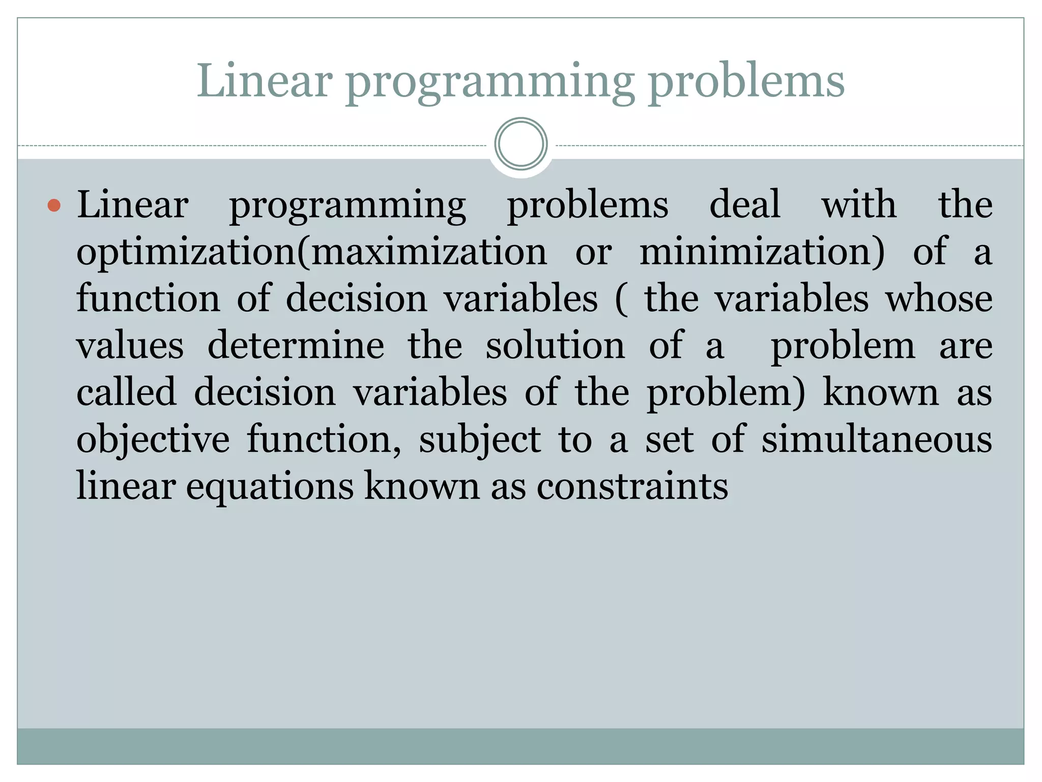
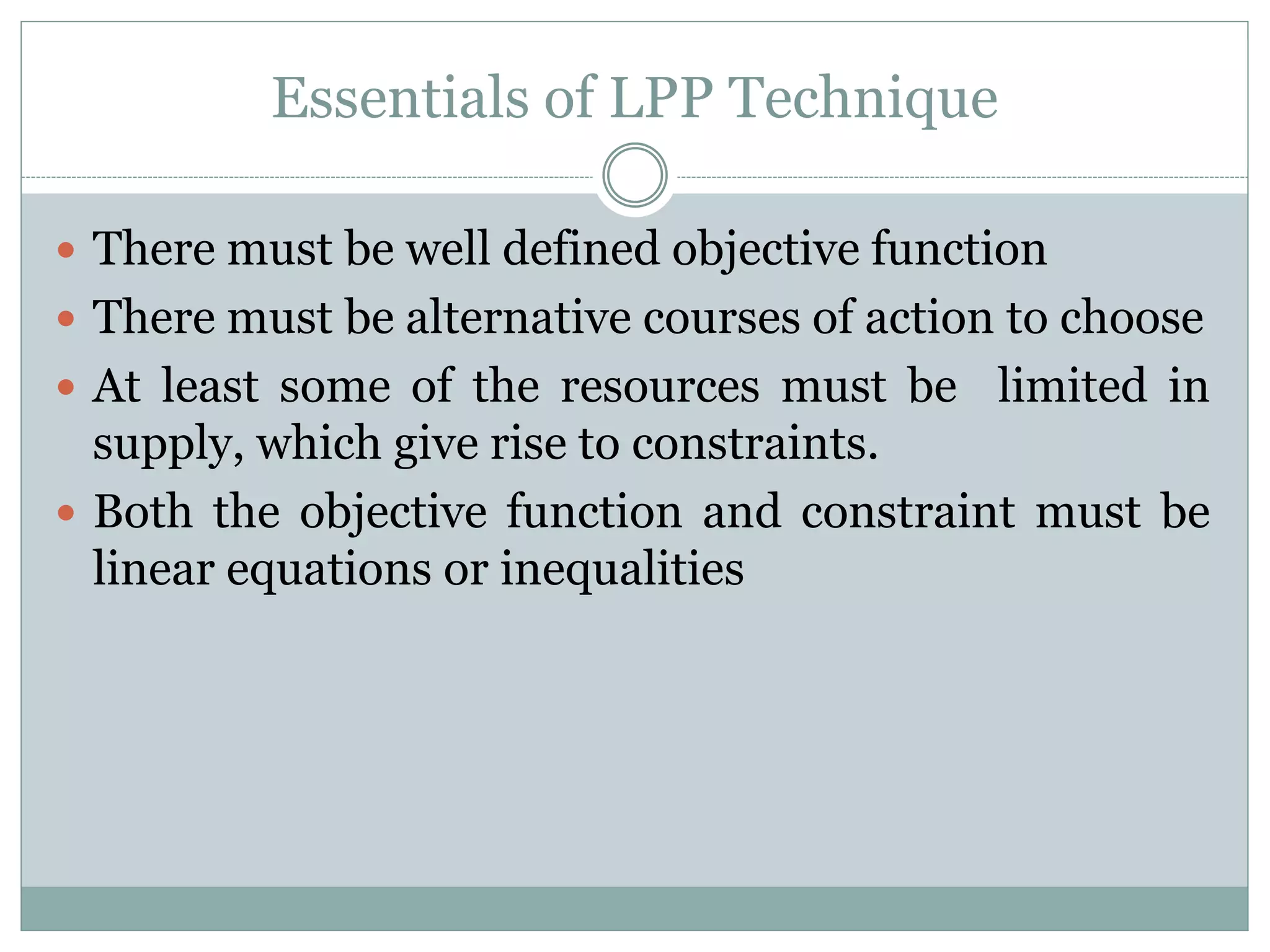
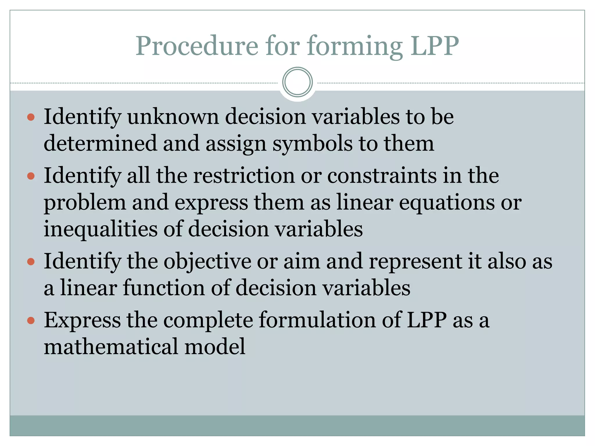
The document discusses different types of mathematical models, including deterministic and probabilistic models. It provides examples of each. It also discusses building, verifying, and refining mathematical models. Additionally, it covers optimization models, their components including objective functions and constraints. Finally, it discusses specific types of optimization models like linear programming, network flow programming, and integer programming.

1. UNIT 1
QUANTITATIVE TECHNIQUES

2. Mathematical Model
 Mathematical modeling is the process of creating a
mathematical representation of some phenomenon in
order to gain a better understanding of that
phenomenon.
 It is a process that attempts to match observation with
symbolic statement.
 During the process of building a mathematical model,
the model will decide what factors are relevant to the
problem and what factors can be de-emphasized.
 Once a model has been developed and used to answer
questions, it should be critically examined and often
modified to obtain a more accurate reflection of the
observed reality of that phenomenon.

3. BUILDING A MATHEMATICAL MODEL
 Identify the problem, define the terms in your
problem, and draw diagrams where appropriate
 Begin with a simple model, stating the
assumptions that you make as you focus on
particular aspects of the phenomenon.
 Identify important variables and constants
and determine how they relate to each other.
 Develop the equation(s) that express the
relationships between the variables and constants.

4. VERIFYING AND REFINING A MODEL
 Is the information produced reasonable?
 Are the assumptions made while developing the
model reasonable?
 Are there any factors that were not considered that
could affect the outcome?
 How do the results compare with real data, if
available?

5. Deterministic Model
 Mathematical model in which outcomes are precisely
determined through known relationships among
states and events, without any room for random
variation.
 In such models, a given input will always produce the
same output, such as in a known chemical reaction.

6. Deterministic Model
 An example of a deterministic model is a calculation
to determine the return on a 5-year investment with
an annual interest rate of 7%, compounded monthly.
The model is just the equation below:
 F = P (1 + r/m) Y
 The inputs are the initial investment (P = $1000),
annual interest rate (r = 7% = 0.07), the
compounding period (m = 12 months), and the
number of years (Y = 5).

7. Deterministic Model
 One of the purposes of a model such as this is to make
predictions and try “What If?” scenarios.
 You can change the inputs and recalculate the model and
you’ll get a new answer.
 You might even want to plot a graph of the future value
(F) vs. years (Y).
 In some cases, you may have a fixed interest rate, but
what do you do if the interest rate is allowed to change?
 For this simple equation, you might only care to know a
worst/best case scenario, where you calculate the future
value based upon the lowest and highest interest rates
that you might expect.

8. Probabilistic Model
 Probabilistic models incorporate random variables
and probability distributions into the model of an
event or phenomenon.
 While a deterministic model gives a single possible
outcome for an event, a probabilistic model gives a
probability distribution as a solution

9. Probabilistic Model-Example
 Weather and Traffic
 Weather and traffic are two everyday occurrences that have inherent
randomness, yet also seem to have a relationship with each other.
 For example, if you live in a cold climate you know that traffic tends to be
more difficult when snow falls and covers the roads.
 We could go a step further and hypothesize that there will be a strong
correlation between snowy weather and increased traffic incidents.
 In order to help analyze our hypothesis, we can create a simple
mathematical model of traffic incidents as a function of snowy weather,
based on known data.
 In the following table, we have accumulated a record of the number of snow
days occurring in a certain locality over the past 10 years, along with the
number of traffic incidents reported to police in the same year.
 A scatter plot of the data can be used to visualize the possible correlation.

10. Probabilistic Model

11. Probabilistic Model
 We see that there is a general trend to the data, with traffic
incidents increasing as the number of snow days increases.
 We have added a linear trend line to the data to highlight this
relationship.
 This linear trend is, in fact, a straight line probabilistic
model of the data. The individual data points do not lie exactly on
the line, and so this linear model is not deterministic.
 There is some error in the predictive ability of our model, as shown
by the vertical lines linking individual points to the linear trend line.
 The magnitude of each of these represents an error in the predictive
ability of our model.
 However, given some allowance for these error terms, this straight
line model seems to reasonably represent the number of traffic
incidents that can be expected to occur in that locality during some
year, given the number of snowy days.

12. Operation Research
 OR is a scientific method of providing executive
departments with a quantitative basis for decisions
regarding the operations under their control. – Morse &
Kimball
 Operations research is a scientific approach to problem
solving for executive management. – H.M. Wagner
 Operations research is an aid for the executive in making
this decisions by providing him with the needed
quantitative information based on the scientific method of
analysis. – C. Kittel

13. Models of OR and Optimization
 Linear Programming
 Network Flow Programming
 Integer Programming
 Nonlinear Programming
 Dynamic Programming
 Stochastic Programming
 Queuing
 Simulation

14. LINEAR PROGRAMMING
 A typical mathematical program consists of a single
objective function, representing either a profit to be
maximized or a cost to be minimized, and a set of
constraints that circumscribe the decision variables.
 In the case of a linear program (LP) the objective
function and constraints are all linear functions of the
decision variables.
 Because of its simplicity, software has been developed
that is capable of solving problems containing millions of
variables and tens of thousands of constraints.
 Countless real-world applications have been successfully
modeled and solved using linear programming
techniques.

15. NETWORK FLOW PROGRAMMING
 The term network flow program describes a type of model that
is a special case of the more general linear program.
 The class of network flow programs includes such problems
as the transportation problem, the assignment
problem, the shortest path problem, the maximum
flow problem, the pure minimum cost flow problem,
and the generalized minimum cost flow problem.
 It is an important class because many aspects of actual
situations are readily recognized as networks and the
representation of the model is much more compact than the
general linear program.
 When a situation can be entirely modeled as a network, very
efficient algorithms exist for the solution of the optimization
problem, many times more efficient than linear programming
in the utilization of computer time and space resources.

16. INTEGER PROGRAMMING
 Integer programming is concerned with optimization
problems in which some of the variables are required
to take on discrete values.
 Rather than allow a variable to assume all real
values in a given range, only predetermined discrete
values within the range are permitted.
 In most cases, these values are the integers, giving
rise to the name of this class of models.

17. NONLINEAR PROGRAMMING
 When expressions defining the objective function or
constraints of an optimization model are not linear,
one has a nonlinear programming model.
 Since nonlinear functions can assume such a wide
variety of functional forms, there are many different
classes of nonlinear programming models.
 In general a nonlinear programming model is much
more difficult to solve than a similarly sized linear
programming model.

18. DYNAMIC PROGRAMMING
 Rather than an objective function and constraints, a DP
model describes a process in terms of states, decisions,
transitions and returns.
 The process begins in some initial state where a decision
is made. The decision causes a transition to a new state.
 Based on the starting state, ending state and decision a
return is realized.
 The process continues through a sequence of states until
finally a final state is reached.
 The problem is to find the sequence that maximizes the
total return.

19. STOCHASTIC PROGRAMMING
 The mathematical programming models, such as
linear programming, network flow programming and
integer programming generally neglect the effects of
uncertainty and assume that the results of decisions
are predictable and deterministic.
 This abstraction of reality allows large and complex
decision problems to be modeled and solved using
powerful computational methods.

20. QUEUING
 This situation is almost always guaranteed to occur
at some time in any system that has probabilistic
arrival and service patterns.
 Tradeoffs between the cost of increasing service
capacity and the cost of waiting customers prevent
an easy solution to the design problem.
 The basic objective in most queuing models is to
achieve a balance between these costs.

21. SIMULATION
 When a situation is affected by random variables it is
often difficult to obtain closed form equations that can be
used for evaluation.
 Simulation is a very general technique for estimating
statistical measures of complex systems.
 A system is modeled as if the random variables were
known. Then values for the variables are drawn
randomly from their known probability distributions.
 Each replication gives one observation of the system
response. By simulating a system in this fashion for many
replications and recording the responses, one can
compute statistics concerning the results.
 The statistics are used for evaluation and design.

22. Basics of Optimization Model
 Optimization model has three main components:
 An objective function. This is the function that needs to be
optimized.
 A collection of decision variables. The solution to the optimization
problem is the set of values of the decision variables for which the
objective function reaches its optimal value.
 Decision Variable:
 A factor over which the decision maker has control;
 also known as a controllable input variable.
 Usually designated by X1, X2, X3…
 A collection of constraints that restrict the values of the decision
variables.
 Decision Constraint: A restrictive condition that may affect the
optimal value for an objective function.

23. Scope and applications of Mathematical Models
Mathematical models are useful in solving :
 Resource allocation problems
 Inventory control problems
 Maintenance and replacement problems
 sequencing and scheduling problems
 Assignment of job to employees in order to maximize total profits or
minimize total cost
 Transportation problems
 Shortest route problem like travelling salesman problem
 Marketing management problems
 Finance management problems
 Production planning and control problems
 Design problems
 Queuing problems

24. Advantages
 Provides a tool for scientific analysis.
 Provides solution for various business problems.
 Enables proper deployment of resources.
 Helps in minimizing waiting and servicing costs.
 Enables the management to decide when to buy and
how much to buy?
 Assists in choosing an optimum strategy.
 Renders great help in optimum resource allocation.
 Facilitates the process of decision making.
 Management can know the reactions of the integrated
business systems.
 Helps a lot in the preparation of future managers

25. Linear programming problems
 Linear programming problems deal with the
optimization(maximization or minimization) of a
function of decision variables ( the variables whose
values determine the solution of a problem are
called decision variables of the problem) known as
objective function, subject to a set of simultaneous
linear equations known as constraints

26. Essentials of LPP Technique
 There must be well defined objective function
 There must be alternative courses of action to choose
 At least some of the resources must be limited in
supply, which give rise to constraints.
 Both the objective function and constraint must be
linear equations or inequalities

27. Procedure for forming LPP
 Identify unknown decision variables to be
determined and assign symbols to them
 Identify all the restriction or constraints in the
problem and express them as linear equations or
inequalities of decision variables
 Identify the objective or aim and represent it also as
a linear function of decision variables
 Express the complete formulation of LPP as a
mathematical model