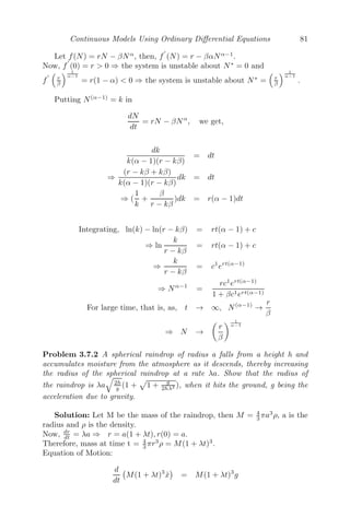
The document describes a textbook on mathematical modeling that covers modeling with all types of differential equations, including ordinary, partial, delay, and stochastic equations. It is a comprehensive textbook that addresses modeling techniques used in analysis. It incorporates MATLAB and Mathematica and includes examples and exercises that can be used for projects. The book is intended for engineers, scientists, and others who use modeling of discrete and continuous systems.

1. Almost every year, a new book on mathematical modeling is published, so, why
another? The answer springs directly from the fact that it is very rare to find a
book that covers modeling with all types of differential equations in one volume.
Until now. Mathematical Modeling: Models, Analysis and Applications covers
modeling with all kinds of differential equations, namely ordinary, partial, delay, and
stochastic. The book also contains a chapter on discrete modeling, consisting of
differential equations, making it a complete textbook on this important skill needed
for the study of science, engineering, and social sciences.
More than just a textbook, this how-to guide presents tools for mathematical
modeling and analysis. It offers a wide-ranging overview of mathematical ideas
and techniques that provide a number of effective approaches to problem solving.
Topics covered include spatial, delayed, and stochastic modeling. The text provides
real-life examples of discrete and continuous mathematical modeling scenarios.
MATLAB®
and Mathematica®
are incorporated throughout the text. The examples
and exercises in each chapter can be used as problems in a project.
Features
• Addresses all aspects of mathematical modeling with mathematical tools used
in subsequent analysis
• Incorporates MATLAB and Mathematica
• Covers spatial, delayed, and stochastic models
• Presents real-life examples of discrete and continuous scenarios
• Includes examples and exercises that can be used as problems in a project
Since mathematical modeling involves a diverse range of skills and tools, the author
focuses on techniques that will be of particular interest to engineers, scientists, and
others who use models of discrete and continuous systems. He gives students a
foundation for understanding and using the mathematics that is the basis of com-
puters, and therefore a foundation for success in engineering and science streams.
K12528
Engineering Mathematics
MATHEMATICAL
MODELING
MATHEMATICAL
MODELING
MATHEMATICAL
MODELING
Models, Analysis and Applications
Models, Analysis and Applications
Sandip Banerjee
Banerjee
K12528_Cover.indd 1 12/18/13 12:21 PM

2. MATHEMATICAL
MODELING
Models, Analysis and Applications
K12528_FM.indd 1 12/10/13 11:42 AM

3. K12528_FM.indd 2 12/10/13 11:42 AM

4. MATHEMATICAL
MODELING
Models, Analysis and Applications
Sandip Banerjee
Indian Institute of Technology
Roorkee
K12528_FM.indd 3 12/10/13 11:42 AM

5. MATLAB® is a trademark of The MathWorks, Inc. and is used with permission. The MathWorks does not
warrant the accuracy of the text or exercises in this book. This book’s use or discussion of MATLAB® soft-
ware or related products does not constitute endorsement or sponsorship by The MathWorks of a particular
pedagogical approach or particular use of the MATLAB® software.
CRC Press
Taylor & Francis Group
6000 Broken Sound Parkway NW, Suite 300
Boca Raton, FL 33487-2742
© 2014 by Taylor & Francis Group, LLC
CRC Press is an imprint of Taylor & Francis Group, an Informa business
No claim to original U.S. Government works
Version Date: 20140110
International Standard Book Number-13: 978-1-4822-2916-5 (eBook - PDF)
This book contains information obtained from authentic and highly regarded sources. Reasonable efforts
have been made to publish reliable data and information, but the author and publisher cannot assume
responsibility for the validity of all materials or the consequences of their use. The authors and publishers
have attempted to trace the copyright holders of all material reproduced in this publication and apologize to
copyright holders if permission to publish in this form has not been obtained. If any copyright material has
not been acknowledged please write and let us know so we may rectify in any future reprint.
Except as permitted under U.S. Copyright Law, no part of this book may be reprinted, reproduced, transmit-
ted, or utilized in any form by any electronic, mechanical, or other means, now known or hereafter invented,
including photocopying, microfilming, and recording, or in any information storage or retrieval system,
without written permission from the publishers.
For permission to photocopy or use material electronically from this work, please access www.copyright.
com (http://www.copyright.com/) or contact the Copyright Clearance Center, Inc. (CCC), 222 Rosewood
Drive, Danvers, MA 01923, 978-750-8400. CCC is a not-for-profit organization that provides licenses and
registration for a variety of users. For organizations that have been granted a photocopy license by the CCC,
a separate system of payment has been arranged.
Trademark Notice: Product or corporate names may be trademarks or registered trademarks, and are used
only for identification and explanation without intent to infringe.
Visit the Taylor & Francis Web site at
http://www.taylorandfrancis.com
and the CRC Press Web site at
http://www.crcpress.com

6. i
To my wife Usha
and
son Aditya
who brought
love and joy
to my life
and to Otso
who taught me
how to do research

8. Contents
1 About Mathematical Modeling 1
1.1 What is Mathematical Modeling? . . . . . . . . . . . . . . . 1
1.2 History of Mathematical Modeling . . . . . . . . . . . . . . . 2
1.3 Importance of Mathematical Modeling . . . . . . . . . . . . 4
1.4 Latest Developments in Mathematical Modeling . . . . . . . 5
1.5 Limitations of Mathematical Modeling . . . . . . . . . . . . 6
2 Mathematically Modeling Discrete Processes 9
2.1 Difference Equations . . . . . . . . . . . . . . . . . . . . . . . 9
2.1.1 Linear Difference Equation with Constant Coefficients 10
2.1.2 Solution of Homogeneous Equations . . . . . . . . . . 10
2.1.3 Difference Equation: Equilibria and Stability . . . . . 14
2.1.3.1 Linear Difference Equation . . . . . . . . . . 14
2.1.3.2 System of Linear Difference Equations . . . . 14
2.1.3.3 Non-Linear Systems . . . . . . . . . . . . . . 16
2.2 Introduction to Discrete Models . . . . . . . . . . . . . . . . 17
2.3 Linear Models . . . . . . . . . . . . . . . . . . . . . . . . . . 18
2.3.1 Population Model Involving Growth . . . . . . . . . . 18
2.3.2 Newton’s Law of Cooling . . . . . . . . . . . . . . . . 19
2.3.3 Bank Account Problem . . . . . . . . . . . . . . . . . 20
2.3.4 Drug Delivery Problem . . . . . . . . . . . . . . . . . 22
2.3.5 Economic Model (Harrod Model) . . . . . . . . . . . . 23
2.3.6 Arms Race Model . . . . . . . . . . . . . . . . . . . . 24
2.3.7 Linear Prey-Predator Problem . . . . . . . . . . . . . 24
2.4 Non-Linear Models . . . . . . . . . . . . . . . . . . . . . . . 27
2.4.1 Density Dependent Growth Models . . . . . . . . . . . 27
2.4.2 The Learning Model . . . . . . . . . . . . . . . . . . . 27
2.5 Miscellaneous Examples . . . . . . . . . . . . . . . . . . . . . 28
2.6 Exercises . . . . . . . . . . . . . . . . . . . . . . . . . . . . . 38
3 Continuous Models Using Ordinary Differential Equations 47
3.1 Introduction to Continuous Models . . . . . . . . . . . . . . 47
3.2 Formation of Various Continuous Models . . . . . . . . . . . 48
3.2.1 Carbon Dating . . . . . . . . . . . . . . . . . . . . . . 48
3.2.2 Drug Distribution in the Body . . . . . . . . . . . . . 49
3.2.3 Growth and Decay of Current in an L-R Circuit . . . 50
iii

9. iv
3.2.4 Rectilinear Motion under Variable Force . . . . . . . . 52
3.2.5 Mechanical Oscillations . . . . . . . . . . . . . . . . . 53
3.2.5.1 Horizontal Oscillations . . . . . . . . . . . . 53
3.2.5.2 Vertical Oscillations . . . . . . . . . . . . . . 54
3.2.5.3 Damped Force Oscillation . . . . . . . . . . . 55
3.2.6 Dynamics of Rowing . . . . . . . . . . . . . . . . . . . 57
3.2.7 Arms Race Models . . . . . . . . . . . . . . . . . . . . 58
3.2.8 Mathematical Model of Influenza Infection (within
Host) . . . . . . . . . . . . . . . . . . . . . . . . . . . 60
3.2.9 Epidemic Models . . . . . . . . . . . . . . . . . . . . . 61
3.3 Steady State Solutions . . . . . . . . . . . . . . . . . . . . . 65
3.4 Linearization and Local Stability Analysis . . . . . . . . . . 66
3.5 Phase Plane Diagrams of Linear Systems . . . . . . . . . . . 68
3.6 Bifurcations . . . . . . . . . . . . . . . . . . . . . . . . . . . 72
3.6.1 Saddle-Node Bifurcation . . . . . . . . . . . . . . . . . 73
3.6.2 Transcritical Bifurcation . . . . . . . . . . . . . . . . . 75
3.6.3 Pitchfork Bifurcation . . . . . . . . . . . . . . . . . . . 77
3.6.4 Hopf Bifurcation . . . . . . . . . . . . . . . . . . . . . 79
3.7 Miscellaneous Examples . . . . . . . . . . . . . . . . . . . . . 80
3.8 Exercises . . . . . . . . . . . . . . . . . . . . . . . . . . . . . 98
4 Spatial Models Using Partial Differential Equations 111
4.1 Introduction . . . . . . . . . . . . . . . . . . . . . . . . . . . 111
4.2 Different Mathematical Models Using Diffusion . . . . . . . . 112
4.2.1 Fluid Flow through a Porous Medium . . . . . . . . . 112
4.2.2 Heat Flow through a Small Thin Rod (One Dimen-
sional) . . . . . . . . . . . . . . . . . . . . . . . . . . . 113
4.2.3 Wave Equation . . . . . . . . . . . . . . . . . . . . . . 115
4.2.4 Vibrating String . . . . . . . . . . . . . . . . . . . . . 117
4.2.5 Traffic Flow . . . . . . . . . . . . . . . . . . . . . . . . 119
4.2.6 Theory of Car-Following . . . . . . . . . . . . . . . . 124
4.2.7 Crimes Model . . . . . . . . . . . . . . . . . . . . . . . 126
4.3 Linear Stability Analysis . . . . . . . . . . . . . . . . . . . . 127
4.3.1 One Species with Diffusion . . . . . . . . . . . . . . . 127
4.3.2 Two Species with Diffusion . . . . . . . . . . . . . . . 128
4.4 A Research Problem: Spatiotemporal Aspect of a Mathematical
Model of Cancer Immune Interaction Considering the Role of
Antibodies . . . . . . . . . . . . . . . . . . . . . . . . . . . . 132
4.4.1 Background of the Problem . . . . . . . . . . . . . . . 132
4.4.2 Spatiotemporal Model Formulation . . . . . . . . . . . 132
4.4.3 Qualitative Analysis . . . . . . . . . . . . . . . . . . . 133
4.4.4 Numerical Results . . . . . . . . . . . . . . . . . . . . 137
4.4.5 Conclusion . . . . . . . . . . . . . . . . . . . . . . . . 138
4.5 Miscellaneous Examples . . . . . . . . . . . . . . . . . . . . . 139
4.6 Exercises . . . . . . . . . . . . . . . . . . . . . . . . . . . . . 148

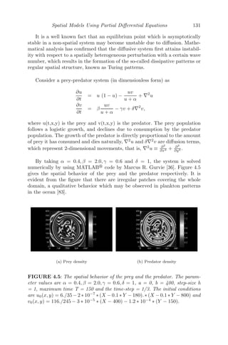
10. v
5 Modeling with Delay Differential Equations 153
5.1 Introduction . . . . . . . . . . . . . . . . . . . . . . . . . . . 153
5.2 Different Models Using Delay Differential Equations . . . . . 154
5.2.1 Delayed Protein Degradation . . . . . . . . . . . . . . 154
5.2.2 Football Team Performance Model . . . . . . . . . . . 155
5.2.3 Breathing Model . . . . . . . . . . . . . . . . . . . . . 156
5.2.4 Housefly Model . . . . . . . . . . . . . . . . . . . . . . 157
5.2.5 Shower Problem . . . . . . . . . . . . . . . . . . . . . 158
5.2.6 Two-Neuron System . . . . . . . . . . . . . . . . . . . 159
5.3 Linear Stability Analysis . . . . . . . . . . . . . . . . . . . . 160
5.3.1 Linear Stability Criteria . . . . . . . . . . . . . . . . . 161
5.4 Miscellaneous Examples . . . . . . . . . . . . . . . . . . . . . 163
5.4.1 A Research Problem: Immunotherapy with Interleukin-
2, a Study Based on Mathematical Modeling [8] . . . . 171
5.4.1.1 Background of the Problem . . . . . . . . . . 171
5.4.1.2 The Model . . . . . . . . . . . . . . . . . . . 173
5.4.1.3 Positivity of the Solution . . . . . . . . . . . 175
5.4.1.4 Linear Stability Analysis with Delay . . . . . 175
5.4.1.5 Estimation of the Length of Delay to Preserve
Stability . . . . . . . . . . . . . . . . . . . . 178
5.4.1.6 Numerical Results . . . . . . . . . . . . . . . 181
5.4.1.7 Conclusion . . . . . . . . . . . . . . . . . . . 182
5.5 Exercises . . . . . . . . . . . . . . . . . . . . . . . . . . . . . 184
6 Modeling with Stochastic Differential Equations 191
6.1 Introduction . . . . . . . . . . . . . . . . . . . . . . . . . . . 191
6.1.1 Probability Space . . . . . . . . . . . . . . . . . . . . . 192
6.1.2 Stochastic Process . . . . . . . . . . . . . . . . . . . . 193
6.1.2.1 Wiener Process (Brownian Motion) . . . . . 194
6.1.3 Stochastic Differential Equation (SDE) . . . . . . . . . 195
6.1.4 Gaussian White Noise . . . . . . . . . . . . . . . . . . 195
6.1.5 Stochastic Stability . . . . . . . . . . . . . . . . . . . . 195
6.2 Some Stochastic Models . . . . . . . . . . . . . . . . . . . . . 196
6.2.1 Stochastic Logistic Growth . . . . . . . . . . . . . . . 196
6.2.2 Heston Model . . . . . . . . . . . . . . . . . . . . . . . 197
6.2.3 Resistor-Inductor-Capacitor(RLC) Electric Circuit with
Randomness . . . . . . . . . . . . . . . . . . . . . . . 197
6.2.4 Two Species Competition Model . . . . . . . . . . . . 199
6.3 A Research Problem: Cancer Self-Remission and Tumor Stabil-
ity - A Stochastic Approach [116] . . . . . . . . . . . . . . . 200
6.3.1 Background of the Problem . . . . . . . . . . . . . . . 200
6.3.2 The Deterministic Model . . . . . . . . . . . . . . . . 202
6.3.3 Equilibria and Local Stability Analysis . . . . . . . . . 203
6.3.4 Biological Implications . . . . . . . . . . . . . . . . . . 205
6.3.5 The Stochastic Model . . . . . . . . . . . . . . . . . . 206

11. vi
6.3.6 Stochastic Stability of the Positive Equilibrium . . . . 207
6.3.7 Numerical Results and Explanations . . . . . . . . . . 211
6.3.8 Concluding Remarks . . . . . . . . . . . . . . . . . . . 211
6.4 Exercises . . . . . . . . . . . . . . . . . . . . . . . . . . . . . 214
7 Hints and Solutions 219
Bibliography 243
Index 253

12. Foreword
When we talk about mathematical modeling it is worthwhile to discuss a
concept of a model that is considerably wider than just the concept of a
mathematical model. It is very difficult, if not impossible, to give a precise
definition of the notion of a model covering the wide spectrum of possibilities.
We shall be satisfied with the following statement: A model is an image of
a sector of reality which is created in order to accomplish a given
task. Consequently the starting point of a modeling process has to be the
identification of the purpose to be satisfied by the model and the task to be
accomplished by the modeling process. This is essential, because it determines
both the sector of reality to be considered and the type of model to be created.
It is important that the model preserves those structures of the real world that
are essential for the goals of the modeling process. It is equally important that
the model does not include unnecessary features. An obvious reason for this
is that otherwise the model may become intractable numerically (if it is a
mathematical model). However, because of the enormous progress made in
computing technology this reason nowadays is in many cases of little impor-
tance. The real, but less obvious, reason is that unnecessary components of a
model may obscure the structure which is important in view of the problem
to solve or they may hide the mechanisms that are essential for the aims of
the modeling process. To determine what is important and has to be included
in a model and what is not important and therefore should be neglected is
the essence of modeling.
Types of Models. The “definition” of a model given above includes a rather
wide range of different types of models including, of course, mathematical
models. Even if we are mainly interested in mathematical models it is useful
to also consider other types of models in order to demonstrate that certain
guidelines should be observed in a modeling process. Below we list a few types
of models:
• Verbal descriptions: Here the sector of reality could be a political event,
like a session of parliament or a demonstration, and the image, i.e., the
model, text in a newspaper. Ideally one would assume that the goal
for writing the article is to give an unbiased report of the event which
captures the politically relevant facts correctly. However, the purpose of
the model (i.e., of the article) could also be different. For example the
text should create the impression in the reader that the event demon-
vii

13. viii
strates the superiority of the program of a certain political party over
the program of another party. Other examples of models in the form of
a verbal description are, for instance, witness reports in the case of a
car accident, or minutes of a meeting.
• Structured lists of measurements: Such lists of measurements or attributes
can also be considered as models, the purpose being to classify certain
objects with sufficient precision for a given purpose. As an example we
mention the numbers arranged in a size chart for blue jeans which allow
clothing manufacturers to produce jeans such that a high percentage of
customers can find jeans that fit.
• Maps of various kinds: Here the sector of reality usually is a part of the
surface of the earth and the image is a geometric two-dimensional struc-
ture. The appearance of a map is clearly dependent on the purpose it
was designed for. A road map looks very different than a physical or a
political map. If one tries to navigate through a city with public buses
using an aerial photograph (which also can be considered as a model
of the city) instead of a map for the bus lines one will realize that the
photograph, though it contains much more detail, is totally unsuited for
the purpose of using buses in the city.
• Real models: These are replicas of real objects which preserve certain ge-
ometric properties or some of the functionality of the real object. As
an example we mention models of aircraft for wind tunnel experiments,
which are down-scaled replicas of real aircraft preserving the shape of
the real aircraft as much detail as possible in order to study the airflow
around the airplane. Another example is provided by dummies as models
for the human body in crash tests. Here the shape and internal structure
of a human body are imitated only to the extent that damages to the
dummy during a crash test allow one to conclude what kind of injuries
a person would have suffered in a car accident of the kind simulated by
the crash test.
• Mathematical models: In this case the image of a part of reality is a math-
ematical structure given, for instance, by a set of linear or nonlinear
equations, by a system of ordinary or partial differential equations, by a
stochastic process etc. Of course, this is the kind of model we are mainly
interested in these notes, and which are the topic of this book.
We can distinguish different types of mathematical models. Examples are:
• Dynamical models: Here, the time behavior of the real system is of prime
interest. Consequently the main components of the model are ordinary
differential equations, delay equations, stochastic differential equations
and/or partial differential equations of parabolic or hyperbolic type, for
instance.

14. ix
• Geometric models: In this case the model should represent the geometry of
the real system. One example is given by models which can be used in
order to optimize the shape of the real system according to given criteria
(minimal weight and still resist forces of a given magnitude without
deformation). Another example is provided by computer tomography or
magnetic resonance imaging in medicine.
• Classifying models: These are models which allow classifying members of a
set of objects or of a population on the basis of available data. Many
statistical models fall into this class.
Goals of a Modeling Process: It was stressed above that the first step
in a modeling process is to give a clear definition of the goal to be achieved
by this process. In the following we provide a list of possible goals, which is
far from being complete:
• Simulations instead of experiments: Compared to numerical simulations ex-
periments are in general much more expensive. Therefore a very common
goal of a modeling process is to replace experiments by numerical sim-
ulations on the basis of a mathematical model. However, that does not
mean that experiments eventually will be replaced completely by numer-
ical simulations. We always shall need experiments in order to validate
a model which has been developed. Besides the cost advantage of nu-
merical simulations with a model another reason for doing simulations
can be that it may be impossible to conduct an experiment because it
is too dangerous or it is prohibited by ethical reasons. Of course in such
a case simulation results have to be considered with great care, because
validation of the model may also be limited.
• Control of processes in the real world: Many processes in the real world have
to be controlled in order to work in a satisfactory way. For instance, the
goal can be to keep the dynamics of a system in a prescribed status de-
spite perturbations which may act on the system. A very simple example
is the temperature control of a room which should keep the temperature
in the room at a given value. Perturbations in this case are caused by
outside temperature changes, changes in the number of people in the
room, opening and closing doors and windows etc. A considerably more
complicated example is provided by an autopilot which should keep an
airplane on a prescribed course. The design of controllers with predefined
properties has to be based on a mathematical model for the process and
the application of results from control theory to that model. Therefore
methods of optimal control and optimization are integral components of
many modeling processes. Of course, control problems arise not only for
technical systems. For instance in disease control it may be necessary to
develop a model in order to design a vaccination strategy to keep the
number of infectious individuals below a given threshold.

15. x
• Models for measurements: Almost all standard measuring devices use some
physical mechanism which relates the quantity to be measured to a
quantity which can be observed directly. For instance, a classical ther-
mometer shows the length of the column of mercury enclosed in a glass
pipe, which is related to the room temperature by two physical pro-
cesses: one is the heat exchange between the air in a room and the
mercury in the thermometer and the other is the fact that the volume
of mercury increases as temperature increases. From this it is also clear
that a classical thermometer cannot follow rapid temperature changes.
From this simple example we should learn that the physical processes on
which the measuring device is based in order to interpret the quality of
the measurements correctly. With the advance of computer technology,
more complex measuring devices frequently implement the numerical al-
gorithms simulating the physical mechanisms on which the functioning
of the device is based. This is already a simple application of mathe-
matical modeling in order to obtain measurements. In more complex
situations models are used in order to ‘measure’ (i.e., to identify) a
quantity which cannot be measured directly by measuring another more
accessible quantity. Such procedures are in particular used in order to
‘measure’ physiological quantities.
• Gain of understanding through mathematical modeling: An important fac-
tor in this context is the fact that mathematical modeling requires a sys-
tematic approach concentrating on the main structural and functional
features of the real system under consideration. This inevitably leads to
a better understanding of the real process.
• Models for educational purposes: Real models have been used for a long
time as teaching devices. With the availability of affordable computing
power in combination with visualization techniques, complex models can
be used to demonstrate the functioning of complex real systems under
varying conditions. In many cases the requirement that the model has
to be validated is relaxed in favor of a more complete representation of
the real system which is at least qualitatively correct.
Validation of a Model: An important concept in mathematical model-
ing is given by the domain of validity of a model. This can be defined as that
sector (time-wise, spatial or functional) of reality that is represented by the
model with sufficient accuracy. Validation of a model requires that simulation
results of the model have to be compared with data from experiments that
may have been performed for the sole purpose of validating the model. This
means that parameters of the model have to be adjusted in order to get an
optimal agreement between simulations and data; i.e., we choose the parame-
ters such that some functional measuring the difference between model output
and data is minimized. The validation step should also check that the origi-
nally defined goals for the modeling process are reached; i.e., if the domain of

16. xi
validity of the model included the sector of reality for which the model was
developed.
Simulations with a model involving substantial changes in the model pa-
rameters in order to predict the behavior of the real system in more extreme
situations has to be done with great care, because the real system correspond-
ing to the changed parameters may not hold true in the domain of validity of
the model.
Guidelines: When one is involved in a modeling process it is important
to observe guidelines which have proven to be helpful for accomplishing the
task. A few of these guidelines are:
• The first step of a modeling process is to identify the sector of reality to be
considered and to establish the goals of the modeling process.
• Next, it is important to determine the mechanisms to be considered, and
the details that should be neglected, using empirical observations and
available knowledge of the real system.
• Variables and parameters of the model should have interpretations in real-
ity. For models that reflect causal mechanisms acting in the real system,
this guideline must be followed. Parameters of model components which
reflect physical, chemical or biological mechanisms need to have an in-
terpretation in the relevant mechanism. This allows interpreting changes
in the parameters as changes in real system and vice versa.
• If a model does not achieve the given goals, then it has to be modified or
abandoned and replaced by a new one. This guideline seems to be ob-
vious. However, mathematicians involved in the modeling process tend
to like a mathematical model that provides an interesting mathematical
structure and the possibility to prove nice theorems. But it may be that
the mathematically interesting model has a rather poor performance
with respect to the goals of the modeling process.
Important Factors in Mathematical Modeling: We want to draw
attention to some important factors for the rapid development and success
of mathematical modeling in various applied sciences. One is the requirement
for precision in control or simulation of more complicated real processes. This
and other needs require mathematical modeling of real processes of increas-
ing complexity also in fields where in the past this was not necessary or not
possible. This has accelerated the interaction between applied sciences and
mathematics and is leading to new mathematical methodologies. Throughout
the history of mathematics, interaction with applications has been an impor-
tant factor for the further development of mathematics per se.

17. xii
Perhaps the most important factor for the rapid development of mathemat-
ical modeling in various applications is the availability of enormous computing
power, which allows considering models of a complexity that was unthinkable
before we had programmable computers. In this context one has to point out
the possibilities for visualizing simulation results provided by modern com-
puters.
An important factor that is quite often underestimated in the context of
mathematical modeling is the introduction of new technologies for measure-
ments and data collection. This is not surprising in view of the needs for data
on a real system for the validation phase of a modeling process.
The Role of Mathematicians: Mathematical modeling not only requires
knowledge of existing mathematical theories or methodologies, but in view of
the rapidly increasing requirements of mathematical models also the devel-
opment of new mathematical methodologies. This is certainly a task where
mathematicians are challenged to contribute their competence and experi-
ence. However, the role of mathematicians in mathematical modeling is not
only to provide the necessary mathematics once the model has been devel-
oped by the applied scientists. In order to be really helpful in a modeling
process the mathematician has to be an integral part of this process. To do
so the mathematician must be able to communicate with the applied scien-
tists on their terms, which means he has to absorb enough of the applied field
to understand the problems and peculiarities of this field. Applied scientists
cannot be expected to enter the relevant mathematical fields to the same de-
gree. Moreover, for cooperation of mathematicians and applied scientists in a
modeling process to be successful mathematicians have to adopt the goals of
the modeling process which is a goal in the applied area. Finally it should be
stressed that mathematicians can add important competencies as partners in
a modeling process because they are trained to attack problems in a formal
and structured approach, which makes it easier for them to neglect unimpor-
tant details and to recognize the underlying structure of a process.
This book reflects most of the points presented here in concrete situations
which in my opinion makes it a valuable contribution to the literature on
mathematical modeling for the target audience of undergraduate students, as
well as for anyone interested in mathematical modeling.
Graz, September 2013 Franz Kappel

18. Preface
Almost every year, a new book on mathematical modeling is published, hence
the inevitable question is: Why another? The answer springs from the fact
that it is rare to find a book that covers modeling with all types of differential
equations in one volume. In my study of books on mathematical modeling
with differential equations, none of them covered all the aspects of differential
equations. It is this that motivated me to write a book on mathematical mod-
eling that will cover modeling with all kinds of differential equations, namely,
ordinary, partial, delay and stochastic. The book also contains a chapter on
discrete modeling, consisting of difference equations. It is this aspect of the
book that makes it unique and complete and is one of its salient features.
Mathematical modeling is an important aspect of the study of science and
engineering. Even social sciences involve mathematical modeling. The primary
aim of the book is to work towards creating in the reader an awareness of the
concepts involved in mathematical modeling so as to build a solid foundation
in the subject. Since mathematical modeling involves a diverse range of skills
and tools, I have focused on techniques that would be of particular interest
to engineers, scientists and others who use models of discrete and continuous
systems. In an age when computers rule, students of engineering and science
will be better placed if they understand and use the mathematics that is the
basis of computers. Mathematics is necessary for engineering and science. This
will remain unaltered in spite of all changes that may come about in computa-
tion. I never tire of telling my students that it is a risky proposition to accept
computer calculations without having recourse to some parallel closed-form
modeling to verify the veracity of the results. Finally, it is fun and satisfying
to do mathematical manipulations that explain how and why things happen.
My target audience is undergraduates who are keen to grasp the basics
of mathematical modeling. Graduate students who want to use mathematical
modeling in their research will also find the book useful. My experience with
books on mathematical modeling has been that they are effective in some ar-
eas of mathematical modeling using a particular kind of differential equation
needed for the model (either ODE/PDE/DDE or even stochastic) but never
consider the complete picture as far as modeling with differential equation is
concerned. It is important for students to recognize the relevance and applica-
tion of their knowledge of mathematics to practical applications. This book, I
xiii

19. xiv
hope, bridges the gap between the student’s abilities and modeling and would
prepare students to venture forth on their own to solve problems on mathe-
matical modeling using differential equations.
It has taken me almost 3 years to complete this book and this experi-
ence has taught me that writing a book is not an easy task. However, the
end result justifies the hard work that goes into it and leaves one with a
sense of satisfaction once it is ready. The amount of knowledge that I have
gained while working on this book is immense and that is reward in itself. The
book is divided into six chapters. The first chapter introduces the subject of
mathematical modeling, its history, possibilities and its limitations. Chapter
2 deals with discrete models using difference equations. Chapter 3, the largest
chapter, discusses modeling with ordinary differential equations and incor-
porates innumerous examples from physics, chemistry, biology, ecology and
engineering. Chapter 4 is concerned with modeling dealing with partial differ-
ential equations including examples on fluid flow, heat flow, traffic flow and
pattern formation. Chapter 5 focuses on delay differential equations, namely,
solving techniques of simple DDE’s and its stability. Examples from physics,
biology, ecology, finance and its numerical solutions have been discussed in
this chapter; a research problem has been included for those interested in
advance mathematical theory of DDE. The effect of stochasticity on popu-
lation dynamics, epidemiology, finance models, tumor-immune interaction is
the highlight of Chapter 6.
Years of teaching the subject have honed my skills in the area of mathe-
matical modeling; however, perfection is something that one ought to strive
for. I am sure I have not yet achieved it, and hence would welcome any sug-
gestion for improvements, comments and criticisms (directly to sandipbaner-
jea@gmail.com) for later editions of the book.
A book is always the product not only of its author, but also various people
who have in their way contributed towards it. Colleagues, research scholars,
the work environment where I teach, the discussions, engagements, discourses
that I have gathered during years of teaching and research, the many confer-
ences, referee reports, seminars, university lectures, training courses, summer
and winter schools, e-mail correspondence, and most importantly, the patience
and constant support of my family. While it would not be possible to name
all those who have helped me on this journey, their contribution has been
immense. I take this opportunity to thank Prof. Hien Tran, North Carolina
State University. During my visit to NCSU, I had full access to their fabu-
lous library which provided me materials so important for research that went
into writing the book. I also thank three anonymous referees who has gone
through my book proposal. Their valuable suggestions have helped me in prop-
erly shaping up the book. I gratefully acknowledge the Quality Improvement
Program (QIP) of IIT Roorkee for providing me financial support for writ-

20. xv
ing the book. My sincere thanks to my research scholars, Ram Keval, Subhas
Khajanchi, Teekam Singh and Sumana Ghosh, who helped me with typing
and proofreading. Special mention is due to Nishi Pulugurtha, who helped me
in the composition of the history of mathematical modeling. Finally, a word
of thanks to my publisher for their active effort in publishing this book.
Sandip Banerjee
Department of Mathematics
Indian Institute of Technology Roorkee
India.
Additional material is available from the CRC web site
http://www.crcpress.com /product/isbn/9781439854518
MATLAB
is a registered trademark of The MathWorks, Inc.
For product information, please contact:
The MathWorks, Inc.
3 Apple Hill Drive
Natick, MA 01760-2098 USA
Tel: 508-647-7000
Fax: 508-647-7001
E-mail: info@mathworks.com
Web: www.mathworks.com

22. Biography
Dr. Sandip Banerjee is Associate Professor in the Department of Math-
ematics, Indian Institute of Technology Roorkee (IITR), India. His areas of
interest are mathematical modeling of interactions between tumors and the
immune system (the spatial aspect and its 3D visualization and validation),
mathematical modeling of hepatitis C, application of stochastic delay differ-
ential equations to population dynamics and tumor modeling, ecological dy-
namics of interacting populations (mainly effects of space and stochasticity),
and stage structured prey-predator models with multiple delays. Mathemat-
ical modeling is his passion. Dr. Banerjee was the recipient of the Indo-US
Fellowship in 2009 and he was awarded IUSSTF Research Fellow medal by
the Indo-US Technology Forum for his contribution to the Indo-US Fellow-
ship 2009 program at the First Indo-US Research Fellowship Conclave, Pune,
India, 15-17 March 2013. In addition to several national and international
projects, Dr. Banerjee is involved in the Virtual Network in Mathematical
Biology project, which promotes mathematical biology in India.
xvii

24. Chapter 1
About Mathematical Modeling
1.1 What is Mathematical Modeling? ........................................ 1
1.2 History of Mathematical Modeling ....................................... 2
1.3 Importance of Mathematical Modeling ................................... 4
1.4 Latest Developments in Mathematical Modeling ......................... 5
1.5 Limitations of Mathematical Modeling ................................... 6
1.1 What is Mathematical Modeling?
Mathematical modeling is the application of mathematics to describe real-
world problems and investigating important questions that arise from it. Using
mathematical tools, the real-world problem is translated to a mathematical
problem, which mimics the real-world problem. A solution to the mathemat-
ical problem is obtained, which is interpreted in the language of real-world
problem to make predictions about the real world.
By real-world problems, I mean problems from biology, chemistry, engi-
neering, ecology, environment, physics, social sciences, statistics, wildlife man-
agement and so on. Mathematical modeling can be described as an activity
which allows a mathematician to be biologist, chemist, ecologist, economist
depending on the problem that he/she is tackling. The primary aim of a
modeler is to undertake experiments on the mathematical representation of a
real-world problem, instead of undertaking experiments in the real world.
Challenges in mathematical modeling
........not to produce the most comprehensive descriptive model but to
produce the simplest possible model that incorporates the major fea-
tures of the phenomenon of interest.
Howard Emmons
1

25. 2 Mathematical Modeling: Models, Analysis and Applications
1.2 History of Mathematical Modeling
Modeling (from Latin modellus) is a way of handling reality. It is the ability
to create models that distinguish human beings from other animals. Models
of real objects and things have been in use by human beings since the Stone
Age as is evident in cave paintings. Modeling became important in the Ancient
Near East and Ancient Greek civilizations. It is writing and counting numbers
which were the first models. Two other areas where modeling was used in its
preliminary forms are astronomy and architecture. By the year 2000 BC, the
three ancient civilizations of Babylon, Egypt and India had a good knowledge
of mathematics and used mathematical models in various spheres of life [117].
In Ancient Greek civilization, the development of philosophy and its close
relation to mathematics contributed to a deductive method, which led to
probably the first instance of mathematical theory. From about 600 BC, ge-
ometry became a useful tool in analyzing reality. Thales predicted the solar
eclipse of 585 BC and devised a method for measuring heights by measuring
the lengths of shadows using geometry. Pythagoras developed the theory of
numbers, and most importantly initiated the use of proofs to gain new re-
sults from already known theorems. Greek philosophers Aristotle, Eudoxus,
and others contributed further and in the next 300 years after Thales, geom-
etry and other branches of mathematics developed further. The zenith was
reached by Euclid of Alexandria who in Circa 300 BC wrote The Elements, a
veritable collection of almost all branches of mathematics known at the time.
This work included, among others, the first precise description of geometry
and a treatise on number theory. It is for this that Euclid’s books became
important for the teaching of mathematics for many hundreds of years, and
around 250 BC Eratosthenes of Cyrene used this knowledge to calculate the
distances between the Earth and the Sun, the Earth and the Moon and the
circumference of the Earth using a geometric model.
A further step in the development of mathematical models was taken up
by Diophantus of Alexandria in about 250 AD, who, in his book Arithmetica,
developed the beginnings of algebra based on symbolism and the idea of a
variable. In the field of astronomy, Ptolemy, influenced by Pythagoras’ idea of
describing celestial mechanics by circles, developed a mathematical model of
the solar system using circles to predict the movement of the sun, the moon,
and the planets. The model was so accurate that it was used until the early
seventeenth century when Johannes Kepler discovered a much more simple
and superior model for planetary motion in 1619. This model, with later re-
finements done by Newton and Einstein, is in use even today.
Mathematical models are used for real-world problems and are hence im-

26. About Mathematical Modeling 3
portant for human development. Mathematical models were developed in
China, India and Persia as well as in the Western world. One of the most
famous Arabian mathematicians was Abu Abd-Allah ibn Musa Al-Hwārizmī,
who lived in the late eighth century [117]. Interestingly, his name still survives
in the word algorithm. His well known books are de numero Indorum (about
the Indian numbers - today called Arabic numbers) and Al-kitab al-muhtasar
fi hisāb al-ǧ abr wa’lmuqābala (a book about the procedures of calculation
balancing) [117]. Both these books contain mathematical models and prob-
lem solving algorithms for use in commerce, survey, and irrigation. The term
algebra was derived from the title of his second book.
In the Western world, it was only in the sixteenth century that mathe-
matics and mathematical models developed. The greatest mathematician in
the Western world after the decline of the Greek civilization was Fibonacci,
Leonardo da Pisa (ca. 1170-ca. 1240). The son of a merchant, Fibonacci made
many journeys to the Orient, and familiarized himself with mathematics as it
had been practiced in the Eastern world. He used algebraic methods recorded
in Al-Hwārizmī’s books to improve his trade as a merchant. He first realized
the great practical advantage of using the Indian numbers over the Roman
numbers which were still in use in Europe at that time. His book Liber Abaci,
first published in 1202, began with a reference to the ten ‘Indian figures’ (0,
1, 2,..., 9), as he called them. 1202 is an important year since this is the year
that saw the number zero being introduced to Europe. The book itself was
meant to be a manual of algebra for commercial use. It dealt in detail with
arithmetical rules using numerical examples which were derived from practical
use, such as their applications in measure and currency conversion.
The painter Giotto (1267-1336) and the Renaissance architect and sculp-
tor Filippo Brunelleschi (1377-1446) are responsible for the development of
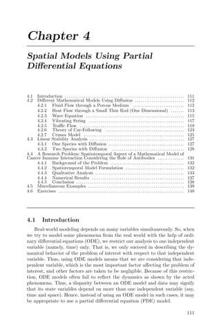
geometric principles. In the later centuries many more and varied mathemati-
cal principles were discovered and the intricacy and complexity of the models
increased. It is important to note that despite the achievements of Diophant
and Al-Hwārizmī, the systematic use of variables was invented by Vieta (1540-
1603) [117]. In spite of all these developments it took many years to realize
the true role of variables in the formulation of mathematical theory. It also
took time for the importance of mathematical modeling to be completely un-
derstood. Physics and its application to nature and natural phenomena is a
major force in mathematical modeling and its further development. Later eco-
nomics became another area of study where mathematical modeling began to
play a major role.

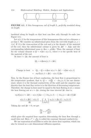
27. 4 Mathematical Modeling: Models, Analysis and Applications
1.3 Importance of Mathematical Modeling
A mathematical model, as stated, is a mathematical description of a real
life situation. So, if a mathematical model can reflect or mimic the behavior
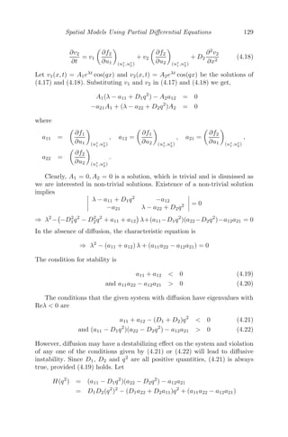
of a real life situation, then we can get a better understanding of the system
through proper analysis of the model using appropriate mathematical tools.
Moreover, in the process of building the model, we discover various factors
which govern the system, factors which are most important to the system and
that reveal how different aspects of the system are related.
The importance of mathematical modeling in physics, chemistry, biology,
economics and even industry cannot be ignored. Mathematical modeling in
basic sciences is gaining popularity, mainly in biological sciences, economics
and industrial problems. For example, if we consider mathematical model-
ing in the steel industry, many aspects of steel manufacture, from mining to
distribution, are susceptible to mathematical modeling. In fact, steel com-
panies have participated in several mathematics-industry workshops, where
they discussed various problems and obtained solution through mathematical
modeling - problems involving control of ingot cooling, heat and mass transfer
in blast furnaces, hot rolling mechanics, friction welding, spray cooling and
shrinkage in ingot solidification, to mention a few [91]. Similarly, mathemati-
cal modeling can be used
(i) to study the growth of plant crops in a stressed environment,
(ii) to study mRNA transport and its role in learning and memory,
(iii) to model and predict climate change,
(iv) to study the interface dynamics for two liquid films in the context of or-
ganic solar cells,
(v) to develop multi-scale modeling in liquid crystal science and many more.
For gaining physical insight, analytical techniques are used. However, to
deal with more complex problems, numerical approaches are quite handy. It
is always advisable and useful to formulate a complex system with a simple
model whose equation yields an analytical solution. Then the model can be
modified to a more realistic one that can be solved numerically. Together with
the analytical results for simpler models and the numerical solution from more
realistic models, one can gain maximum insight into the problem.

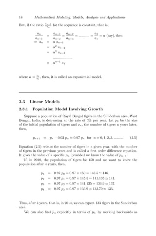
28. About Mathematical Modeling 5
1.4 Latest Developments in Mathematical Modeling
Mathematical modeling is an area of great development and research. In re-
cent years, mathematical models have been used to validate hypotheses made
from experimental data, and at the same time the designing and testing of
these models has led to testable experimental predictions. There are impres-
sive cases in which mathematical models have provided fresh insight into bi-
ological systems, physical systems, decision making problems, space models,
industrial problems, economical problems and so forth. The development of
mathematical modeling is closely related to significant achievements in the
field of computational mathematics.
Consider a new product being launched by a company. In the development
process, there are critical decisions involved in its launch such as timing, de-
termining price, launch sequence, etc. Experts use and develop mathematical
models to facilitate such decision making. Similarly, in order to survive market
competition, cost reduction is one of the main strategies for a manufacturing
plant, where a large amount of production operation costs are involved. Proper
layout of equipment can result in a huge reduction in such costs. This leads to
dynamic facility layout problem for finding equipment sites in manufacturing
environments, which is one of the developing areas in the field of mathematical
modeling [122].
Mathematical modeling also intensifies the study of potentially deadly flu
viruses from mother nature and bio-terrorists. Mathematical models are also
being developed in optical sciences [6], namely, diffractive optics, photonic
band gap structures and wave guides, nutrient modeling, studying the dynam-
ics of blast furnaces, studying erosion, and prediction of surface subsidence.
In geosciences, mathematical models have been developed for talus. Talus
is defined by Rapp and Fairbridge [103] as an accumulation of rock debris
formed close to mountain walls, mainly through many small rockfalls. Hiroyuki
and Yukinori [90] have constructed a new mathematical model for talus devel-
opment and retreat of cliffs behind the talus, which was later applied to the
result of a field experiment for talus development at a cliff composed of chalk.
They developed the model which was in agreement with the field observations.
There has been tremendous development in the interdisciplinary field of
applied mathematics in human physiology in the last decade, and development
continues. One of the main reasons for this development is the researcher’s im-
proved ability to gather data, whose visualization have much better resolution
in time and space than just a few years ago. At the same time, this devel-
opment also constitutes a giant collection of data as obtained from advanced

29. 6 Mathematical Modeling: Models, Analysis and Applications
measurement techniques. Through statistical analysis, it is possible to find
correlations, but such analysis fails to provide insight into the mechanisms
responsible for these correlations. However, when it is combined with mathe-
matical modeling, new insights into the physiological mechanisms are revealed.
Mathematical models are being developed in the field of cloud computing
to facilitate the infrastructure of computing resources in which large pools of
systems (or clouds) are linked together via the internet to provide IT services
(for example, providing secure management of billions of online transactions)
[25]. Development of mathematical models are also noticed
(i) in the study of variation of shielding gas in GTA welding,
(ii) for prediction of aging behavior for Al-Cu-Mg/Bagasse Ash particular
composites,
(iii) for public health decision making and estimations,
(iv) for developing of cerebral cortical folding patterns which have fascinated
scientists with their beauty and complexity for centuries,
(v) to predict sunflower oil expression,
(vi) in the development of a new three dimensional mathematical ionosphere
model at the European Space Agency/European Space Operators Centre,
(vii) in battery modeling or mathematical description of batteries, which plays
an important role in the design and use of batteries, estimation of battery pro-
cesses and battery design. These are some areas where mathematical modeling
plays an important role. However, there are many more areas of application.
1.5 Limitations of Mathematical Modeling
Sometimes although the mathematical model used is well adapted to the
situation at hand, it may give unexpected results or simply fail. This may
be an indication that we have reached the limit of the present mathematical
model and must look for a new refinement of the real-world or a new the-
oretical breakthrough [10]. A similar type of problem was addressed in [6],
which deals with Moire theory, involving the mathematical modeling of the
phenomena that occur in the superposition of two or more structures (line
gratings, dot screens, etc.), either periodic or not.
In mathematical modeling, more assumptions must be made, as infor-
mation about real-world systems become less precise or harder to measure.
Modeling becomes a less precise endeavor as it moves away from physical
systems towards social systems. For example, modeling an electrical circuit
is much more straightforward than modeling human decision making or the
environment. Since physical systems usually do not change, reasonable past

30. About Mathematical Modeling 7
information about a physical system is quite valuable in modeling future per-
formance. However, both social systems and environments often change in
ways that are not of the past, and even correct information may be of less
value in forming assumptions. Thus, to understand a model’s limitations, it
is important to understand the basic assumptions that were used to create it.
Real-world systems are complex and a number of interrelated components
are involved. Since models are abstractions of reality, a good model must try to
incorporate all critical elements and interrelated components of the real-world
system. This is not always possible. Thus, an important inherent limitation
of a model is created by what is left out. Problems arise when key aspects of
the real-world system are inadequately treated in a model or are ignored to
avoid complications, which may lead to incomplete models. Other limitations
of a mathematical model are that they may assume the future will be like the
past, input data may be uncertain or the usefulness of a model may be limited
by its original purpose.
However, despite all these limitations and pitfalls, a good model can be
formulated, if a modeler asks himself/herself the following questions about the
model:
(i) Does the structure of the model resemble the system being modeled?
(ii) Why is the selected model appropriate to use in a given application?
(iii) How well does the model perform?
(iv) Has the model been analyzed by someone other than the model authors?
(v) Is adequate documentation of the model available for all who wish to study
it?
(vi) What assumptions and data were used in producing model output for the
specific application?
(vii) What is the accuracy of the model output?
One should not extrapolate the model beyond the region of fit. A model
should not be applied unless one understands the simplifying assumptions
on which it is based and can test their applicability. It is also important to
understand that the model is not the reality and one should not distort reality
to fit the model. A discredited model should not be retained and one should
not limit himself to a single model, as more than one model may be useful for
understanding different aspects of the same phenomenon. It is imperative to
be aware of the limitations inherent in models. There is no best model, only
better models.

32. Chapter 2
Mathematically Modeling Discrete
Processes
2.1 Difference Equations ...................................................... 9
2.1.1 Linear Difference Equation with Constant Coefficients ........... 10
2.1.2 Solution of Homogeneous Equations .............................. 10
2.1.3 Difference Equation: Equilibria and Stability ..................... 14
2.1.3.1 Linear Difference Equation .............................. 14
2.1.3.2 System of Linear Difference Equations .................. 14
2.1.3.3 Non-Linear Systems ..................................... 16
2.2 Introduction to Discrete Models .......................................... 17
2.3 Linear Models ............................................................. 18
2.3.1 Population Model Involving Growth .............................. 18
2.3.2 Newton’s Law of Cooling ......................................... 19
2.3.3 Bank Account Problem ........................................... 20
2.3.4 Drug Delivery Problem ........................................... 22
2.3.5 Economic Model (Harrod Model) ................................. 23
2.3.6 Arms Race Model ................................................. 24
2.3.7 Linear Prey-Predator Problem .................................... 24
2.4 Non-Linear Models ........................................................ 27
2.4.1 Density Dependent Growth Models ............................... 27
2.4.2 The Learning Model .............................................. 27
2.5 Miscellaneous Examples ................................................... 28
2.6 Exercises .................................................................. 38
2.1 Difference Equations
The term difference equation sometimes refers to a specific type of recur-
rence relation. However, difference equation is frequently used to refer to any
recurrence relation.
Let us now see how a difference equation is formulated. Consider the rela-
tion un = cn − 3, where c is an arbitrary constant. Now, un+1 = c(n + 1) − 3.
The required difference equation is obtained by eliminating c from un and
un+1, which gives
un+1 =
un + 3
n
(n + 1) − 3
⇒ nun+1 = (n + 1)un + 3
9

33. 10 Mathematical Modeling: Models, Analysis and Applications
2.1.1 Linear Difference Equation with Constant Coefficients
Consider the linear difference equation of the form
c0un + c1un−1 + c2un−2 = f(n) (2.1)
The difference equation is homogeneous if f(n) = 0, otherwise it is non-
homogeneous. The order of the difference equation is the difference between
the largest and smallest arguments appearing in the difference equation with
unit interval. Thus, the order of equation (2.1) is 2.
Equation (2.1) is a linear difference equation with constant coefficients as
the coefficients of the successive differences are constants and the differences
of successive orders are of first degree. Thus,
c0un + c1(un−1)2
+ c2un−2 = f(n)
is a non-linear difference equation.
2.1.2 Solution of Homogeneous Equations
(a) Consider the first order homogeneous linear difference equation
un − k(un−1) = 0 (2.2)
Putting n = 1,2,3,........... we get,
u1 = ku0
u2 = ku1 = k2
u0
u3 = ku2 = k3
u0
− − − − − − − − − − −
Thus, un = kn
u0 = ckn
(say)
where c is an arbitrary constant, is a general solution of (2.2).
(b) Consider the first order linear difference equation of the form
un = aun−1 + b = 0 (n = 0,1,2,........), where a and b are constants.
= a(aun−2 + b) + b = a2
xn−2 + b(a + 1)
= a2
(aun−3 + b) + b(a + 1) = a3
xn−3 + b(a2
+ a + 1)
= .......................................
= an
u0 + b(an−1
+ an−2
+ ....... + a2
+ a + 1)
= an
u0 + nb (if a = 1)
= an
u0 + b
1 − an
1 − a
(if a 1)
= an
u0 + b
an
− 1
a − 1
(if a 1),

34. Mathematically Modeling Discrete Processes 11
which is the required solution of the first order linear difference equation
un = aun−1 + b
(c) Consider the second order homogeneous linear difference equation
a0un + a1un−1 + a2un−2 = 0 (2.3)
Assuming the solution of the form un = ckn
(c = 0) and putting it in
(2.3), we get,
a0k2
+ a1k + a2 = 0
⇒ a0k2
+ a1k + a2 = 0 (since, cn
= 0),
which is called the auxiliary equation.
(i) If the auxiliary equation has two distinct real roots, m1 and m2 (say),
then,
c1mn
1 + c2mn
2
is the general solution of (2.3), and c1 and c2 are arbitrary constants.
(ii) If the roots of the auxiliary equation are real and equal, m1 = m2 = m
(say), then,
(c1 + c2n)mn
is the general solution of (2.3), and c1 and c2 are arbitrary constants.
(iii) If the auxiliary equation has imaginary roots (which occur in conju-
gate pairs), α + iβ and α − iβ (say), then,
rn
(c1 cos nθ + c2 sin nθ)
is the general solution of (2.3), r =
α2 + β2 and θ = tan−1
(β
α ), and c1 and
c2 are arbitrary constants.
Note: Solutions for non-homogeneous equations can be obtained by partic-
ular integral methods, undetermined coefficients, Z-Transform, Laplace Trans-
form etc. Interested readers can look into [27, 43, 80] for detailed information.
Example 2.1.1 Obtain the difference equation by eliminating the arbitrary
constants from un = A2n
+ B(−3)n
.
Solution: Given,
un = A2n
+ B(−3)n
⇒ un+1 = A2n+1
+ B(−3)n+1
⇒ un+2 = A2n+2
+ B(−3)n+2

35. 12 Mathematical Modeling: Models, Analysis and Applications
Therefore,
un+1 = 2A2n
− 3B(−3)n
un+2 = 4A2n
+ 9B(−3)n
Solving, we get
A =
3un+1 + un+2
102n
and B =
un+2 − 2un+1
15(−3)n
Thus, the required difference equation is
un =
3un+1 + un+2
10
+
un+2 − 2un+1
15
⇒ un+2 + un+1 − 6un = 0.
Example 2.1.2 Find un if u0 = 0, u1 = 1 and un+2 + 16un = 0.
Solution: Let un = kn
(k = 0) be a solution of un+2 + 16un = 0, then the
required auxiliary equation is
k2
+ 16 = 0
⇒ k = ±4i
The general solution is
un = c1(4i)n
+ c2(−4i)n
= 4n
[c1einπ/2
+ c2e−inπ/2
]
= 4n
[A1 cos(nπ/2) + A2 sin(nπ/2)]
where A1 and A2 are arbitrary constants. Now, u0 = 0 and u1 = 1 implies
A1 = 0 and A2 = 1
4 . Therefore,
un = 4n−1
sin(nπ/2)
is the required solution.
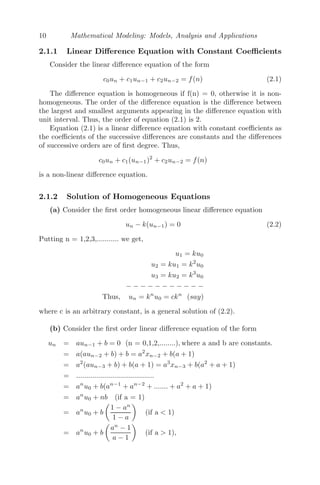
Note: The solutions of homogeneous linear difference equations with con-
stant coefficients are composed of linear combinations of the basic expressions
of the form un = ckn
. The qualitative behavior of the basic solution will
depend on the real values of k, namely, on the four possible ranges [26]:
k ≥ 1, k ≤ −1, 0 k 1, − 1 k 0
For k ≥ 1, the solution un = ckn
becomes unbounded as n increases;
for 0 k 1, kn
goes to zero as n increases, hence un decreases; for −1

36. Mathematically Modeling Discrete Processes 13
k 0, kn
oscillates between positive and negative values, with diminishing
magnitude to zero and for k −1, kn
oscillates between positive and negative
values with increasing magnitude.
The marginal points k = 1, k = 0 and k = −1 correspond to constant
solution (un = c), zero solution (un = 0) and an oscillatory solution between
−c and +c respectively. Figure 2.1 illustrates different behaviors for different
ranges of k.
2 4 6 8
n
100
100
200
un
2 4 6 8
n
0.4
0.2
0.2
0.4
0.6
0.8
1.0
un
2 4 6 8
n
0.2
0.4
0.6
0.8
1.0
un
2 4 6 8
n
50
100
150
200
250
un
FIGURE 2.1: The qualitative behavior of un = Ckn
for different ranges of
k, namely, −1 ≤ k ≤ 1.
Example 2.1.3 Solve: xn+1 = xn
4 + yn, yn+1 = 3xn
16 − yn
4 .
Solution:
xn+1 =
xn
4
+ yn ⇒ yn = xn+1 −
xn
4
⇒ yn+1 = xn+2 −
xn+1
4
Eliminating yn+1 from both the equations, we get,
4xn+2 − xn = 0
The required auxiliary equation is
4k2
− 1 = 0
⇒ k = ±
1
2
The general solution is
xn = c1
1
2
n
+ c2
−1
2
n

37. 14 Mathematical Modeling: Models, Analysis and Applications
where c1 and c2 are arbitrary constants. Similarly, it can be shown,
yn = d1
1
2
n
+ d2
−1
2
n
where d1 and d2 are arbitrary constants.
2.1.3 Difference Equation: Equilibria and Stability
2.1.3.1 Linear Difference Equation
We consider an autonomous linear discrete equation of the form un =
aun−1 + b (a = 1). If u∗
be the equilibrium solution of the model, then
un = un−1 = u∗
(there is no change from generation n-1 to generation n)
⇒ au∗
+ b = u∗
⇒ u∗
=
b
1 − a
.
The equilibrium point u∗
is said to be stable if all the solutions of
un = aun−1 + b approach u∗
= b
1−a as n becomes large (→ ∞). The equilib-
rium point u∗
is unstable if all solutions (if exists) diverge from u∗
to ±∞.
The stability of the equilibrium solution u∗
of the equation un = aun−1 + b
depends on a. It is stable if |a| 1 and unstable if |a| 1. We reach an
ambiguous case if a = ±1.
2.1.3.2 System of Linear Difference Equations
For a system of difference equations, it is possible to determine the stability
of the system using eigenvalues. We consider the homogeneous system,
un+1 = αun + βvn
vn+1 = γun + δvn
which can be expressed in the matrix form as,
un+1
vn+1
=
α β
γ δ
un
vn
⇒ wn+1 = Awn where wn =
un
vn
and A =
α β
γ δ
.
Clearly (0, 0) is the equilibrium point of the homogeneous system.

38. Mathematically Modeling Discrete Processes 15
Theorem 2.1.3.1 Let λ1 and λ2 be two real distinct eigenvalues of the coef-
ficient matrix A of a homogeneous linear system. Then, the equilibrium point
(0, 0) is
(i) stable if both | λ1 | 1 and | λ2 | 1
(ii) unstable if both | λ1 | 1 and | λ1 | 1
(iii) saddle if | λ1 | 1 and | λ1 | 1 or if | λ1 | 1 | λ1 | 1
Note: Please note that λ1 = λ2 = 1 is a rare borderline case and will not be
considered here.
Theorem 2.1.3.2 Let λ1 = λ2 = λ∗
be a real and equal eigenvalue of the
coefficient matrix A of the homogeneous linear system, then the equilibrium
point (0, 0) is
(i) stable if |λ∗
| 1
(ii) unstable if |λ∗
| 1
Theorem 2.1.3.3 Let a + ib and a − ib be the complex conjugate eigenvalues
of the coefficient matrix A of a homogeneous linear system, then the equilib-
rium point (0, 0) is
(i) stable if |a ± ib| 1
(ii) unstable if |a ± ib| 1
For a non-homogeneous linear system of the form wn+1 = Awn + b where
wn =
un+1
vn+1
and A =
α β
γ δ
and b =
k1
k2
, the equilibrium solu-
tion is given by un+1 = un = u∗
and vn+1 = vn = v∗
.
For stability, the same results hold as for the homogeneous system. This is
due to the fact that the non-homogeneous system, with a unique equilibrium
point, can be converted to a homogeneous system. If w∗
= (u∗
, v∗
) be the
equilibrium point of the non-homogeneous system
un+1 = αun + βvn + k2
vn+1 = γun + δvn + k2
then
u∗
= αu∗
+ βv∗
+ k1
v∗
= γv∗
+ δv∗
+ k2
⇒ w∗
= Aw∗
+ b
⇒ Aw∗
− w∗
+ b = 0 (null matrix)
Substituting wn = zn + w∗
in wn+1 = Awn + b we get,

39. 16 Mathematical Modeling: Models, Analysis and Applications
zn+1 + w∗
= A(zn + w∗
) + b
⇒ zn+1 = Azn + Aw∗
− w∗
+ b
⇒ zn+1 = Azn (since Aw∗
− w∗
+ b = 0),
which is a homogeneous system, whose stability has already been discussed.
2.1.3.3 Non-Linear Systems
Non-linear difference equations are to be handled with special techniques
and cannot be solved by simply setting un = kn
. Here, we shall not discuss
about the solutions of non-linear difference equations but focus on the quali-
tative behaviors, namely, steady state and stability.
In the context of difference equations, x∗
is the steady state solution (equi-
librium solution) of the non-linear difference equation
xn+1 = f(xn), if xn+1 = xn = x∗
that is, there is no change from generation n to generation (n+1).
By definition, the steady state solution is stable if for 0, ∃ a δ 0 such
that |x0 − x∗
| δ implies that for all n 0, |fn
(x0) − x∗
| . The steady
state solution is asymptotically stable if, in addition, limx→∞ xn = x∗
holds.
Once we have obtained the steady state solution, we look into its stability,
that is, given some value xn close to x∗
, does xn tends towards x∗
or move
away from it? To address this issue, we give a small perturbation to the system
about the steady state x∗
. Mathematically, this means replacing xn by x∗
+ n,
where n is small. Then,
xn+1 = f(xn)
⇒ x∗
+ n+1 = f(x∗
+ n)
≈ f(x∗
) + nf
(x∗
) (by Taylor series expansion)
= x∗
+ nf
(x∗
)
Since x∗
is the equilibrium solution, x∗
= f(x∗
), which implies
n+1 ≈ nf
(x∗
) (2.4)
The solution of (2.4) will decrease if |f
(x∗
)| 1 and increase if |f
(x∗
)|
1 [80].
Theorem 2.1.3.4 The steady state solution x∗
of xn+1 = f(xn) is stable if
|f
(x∗
)| 1 and unstable if |f
(x∗
)| 1

40. Mathematically Modeling Discrete Processes 17
The stability analysis of a non-linear discrete system of the form un+1 =
f(un, vn) and vn+1 = g(un, vn) near the equilibrium point (u∗
, v∗
) can be
determined by linearizing the system about the equilibrium point.
Theorem 2.1.3.5 Let (u∗
, v∗
) be an equilibrium solution of non-linear sys-
tems un+1 = f(un, vn) and vn+1 = g(un, vn) and A is the corresponding
matrix of partial derivatives given by A =
fx(u∗
, v∗
) fy(u∗
, v∗
)
gx(u∗
, v∗
) gy(u∗
, v∗
)
, then
(u∗
, v∗
) is stable if each eigenvalue of A has modulus less than 1 and unstable
if one of the eigenvalues of A has modulus greater than 1 [80].
2.2 Introduction to Discrete Models
In discrete models, the state variables change only at a countable num-
ber of points in time. These points in time are the ones at which the event
occurs/change in state. Thus, in discrete time modeling, there is a state tran-
sition function which computes the state at the next time instant given the
current state and input. The changes are really discrete in many situations
which occur at well defined time intervals. Moreover, in many cases, the data
are usually discrete rather than continuous. Hence, due to the limitations of
the available data, we may be compelled to work with the discrete model,
even though the underlying model is continuous.
Consider a sequence a1, a2, a3, ..........., an, ........ .
Let the differences an+1 − an = constant = k (say), for the sequence, then
an − an−1 = an−1 − an−2 = an−2 − an−3 = ........... = a2 − a1 = k
⇒ an = an−1 + k
= an−2 + 2k
= an−3 + 3k
....................
= a1 + (n − 1)k
Thus, an is a linear function of n and is called a linear model.

41. 18 Mathematical Modeling: Models, Analysis and Applications
But, if the ratio an+1
an
for the sequence is constant, that is,
an
an−1
=
an−1
an−2
=
an−2
an−3
= ........... =
a2
a1
= α (say), then
⇒ an = α an−1
= α2
an−2
= α3
an−3
....................
= αn−1
a1
where α = a2
a1
, then, it is called an exponential model.
2.3 Linear Models
2.3.1 Population Model Involving Growth
Suppose a population of Royal Bengal tigers in the Sunderban area, West
Bengal, India, is decreasing at the rate of 3% per year. Let p0 be the size
of the initial population of tigers and xn, the number of tigers n years later,
then,
pn+1 = pn − 0.03 pn = 0.97 pn for n = 0, 1, 2, 3, .......... (2.5)
Equation (2.5) relates the number of tigers in a given year, with the number
of tigers in the previous years and is called a first order difference equation.
It gives the value of a specific pn, provided we know the value of pn−1.
If, in 2010, the population of tigers be 150 and we want to know the
population after 4 years, then,
p1 = 0.97 p0 = 0.97 × 150 = 145.5 146.
p2 = 0.97 p1 = 0.97 × 145.5 = 141.135 141.
p3 = 0.97 p2 = 0.97 × 141.135 = 136.9 137.
p4 = 0.97 p3 = 0.97 × 136.9 = 132.79 133.
Thus, after 4 years, that is, in 2014, we can expect 133 tigers in the Sunderban
area.
We can also find p4 explicitly in terms of p0, by working backwards as

42. Mathematically Modeling Discrete Processes 19
follows:
p4 = (0.97) p3
= (0.97) (0.97) p2 = (0.97)2
p2
= (0.97)2
(0.97) p1 = (0.97)3
p1
= (0.97)3
(0.97) p0 = (0.97)4
p0
Thus, we conclude that p4 can be computed without reference to any of the
values p3, p2 and p1, provided we know p0. The general solution of the dif-
ference equation of the form xn+1 = kxn
(n = 0,1,2,3,......) is xn+1 = kn
x0,
where k = 0.97 in this case. Figure 2.2 shows that for this value of k, the tiger
population will become extinct in approximately 165 years.
50 100 150
Time
20
40
60
80
100
120
140
Number of Tigers
FIGURE 2.2: Royal Bengal tigers will be extinct in approximately 165 years
for k = 0.97.
2.3.2 Newton’s Law of Cooling
Suppose a cup of coffee, initially at a temperature of 190 ◦
F is placed in
a room, which is held at a constant temperature of 70 ◦
F. After 1 minute,
the coffee has cooled to 180 ◦
F. If we need to find the temperature of the
coffee after 15 minutes, we will use Newton’s law of cooling, which states
that the rate of change of the temperature of an object is proportional to the
difference between its own temperature and the ambient temperature (i.e. the
temperature of its surroundings). Mathematically, this means,
tn+1 − tn = k(S − tn)
where tn is the temperature of the coffee after n minutes, S is the temperature
of the room and k is the constant of proportionality.

43. 20 Mathematical Modeling: Models, Analysis and Applications
We first make use of the information given about the change in the tempera-
ture of the coffee during the first minute to determine the value of the constant
of proportionality k. Then,
t1 − t0 = k(S − t0)
⇒ 180 − 190 = k(70 − 190)
⇒ k =
1
12
⇒ tn+1 − tn =
1
12
(70 − tn)
⇒ tn+1 =
11
12
tn +
70
12
This is of the form (2.1.2 b), whose solution is given by
tn =
11
12
n
190 + 70
1 −
11
12
n
= 70 + 120
11
12
n
, for n = 0,1,2,......... .
For n = 15,
t15 = 70 + 120
11
12
15
= 102.54
Hence, after 15 minutes, the coffee has cooled to just under 103 ◦
F.
Also, limn→∞
11
12
n
= 0, which implies that the temperature of the coffee
will approach the equilibrium temperature of 70 ◦
F, the room temperature as
n increases (see Figure 2.3).
2.3.3 Bank Account Problem
Suppose a savings account is opened that pays 4% interest compounded
yearly with initial deposit of Rs. 10000.00 (Indian Rupees) and a deposit of
Rs. 5000.00 is made at the end of each year. For a savings account that is
compounded yearly, the interest is added to the principal at the end of each
year. If an is the amount at the end of year n (n = 0, 1, 2, 3......), then
a1 = a0 + ra0 = (1 + r)a0
a2 = a1 + ra1 = (1 + r)a1
.........................................
.........................................
an+1 = an + ran = (1 + r)an
where r is the rate of interest. Now, if a deposit of Rs. 5000.00 is made at
the end of each year, then the dynamic model which describes this scenario is

44. Mathematically Modeling Discrete Processes 21
20 40 60 80 100
Time
50
100
150
Temperature
FIGURE 2.3: The cup of coffee initially at 190 ◦
F reaches the room temper-
ature of 70 ◦
F as n increases.
given by
an+1 = (1 + r)an + 5000 = (1 + 0.04)an + 5000 = 1.04an + 5000
Thus the amount for three consecutive years will be
a1 = 1.04a0 + 5000 = 1.04 × 10000 + 5000 = 10400 + 5000 = 15400
a2 = 1.04 × 15400 + 5000 = 16016 + 5000 = 21016
a3 = 1.04 × 21016 + 5000 = 21856.64 + 5000 = 26856.64
and so on. Let us now consider a different scenario, where no deposits are
made but Rs. 2000.00 is withdrawn at the end of each year. We want to find
out how much money be deposited, so that we never run out of cash. The
model for this scenario is
an+1 = 1.04an − 2000,
where we assume that the money is withdrawn after the interest from previous
years has been added and we are not penalized for withdrawing money each
year. The equilibrium value for this is given by
an+1 = an = a∗
n
⇒ 1.04a∗
n − 2000 = a∗
n
⇒ a∗
n =
2000
0.04
= 50000.00
Thus, if the initial deposit (a0) in the account is Rs. 50000.00 and we withdraw
Rs. 2000 each year, then the account will always have the same amount at the
end of each year (see Figure 2.4).

45. 22 Mathematical Modeling: Models, Analysis and Applications
An obvious question is what happen if a0 50000 or a0 50000. Figure
2.4 shows that if a0 is less that 50000, the amount in the account decreases to
zero and the amount grows without bound if a0 is greater than 50000. Thus
the system approaches zero or increases without bound if a0 = 50000 and
therefore this equilibrium value is unstable.
10 20 30 40
Time
20000
40000
60000
80000
100000
Amount in Rupees
FIGURE 2.4: The amount of money as time increases when the initial de-
posits a0 50000, a0 = 50000 and a0 50000.
2.3.4 Drug Delivery Problem
Suppose a patient is given a drug to treat some infection. The amount of
drug in the patient’s bloodstream decreases at the rate of 50% per hour. To
sustain the drug to a certain level, an injection is given at the end of each
hour that increases the amount of drug in the bloodstream by 0.2 unit. The
dynamic model which describes this scenario is given by
an+1 = 0.5an + 0.2
where an is the amount of drug in the blood at the end of each hour.
The equilibrium solution of this model is given by
an+1 = an = a∗
⇒ 0.5a∗
n + 0.2 = a∗
⇒ a∗
= 0.4
The long-term behavior of the system will depend on the initial value a0.
The figure shows that no matter what is the value of a0, the system always
approaches the value of 0.4, implying that 0.4 is a stable equilibrium (see
Figure 2.5).

46. Mathematically Modeling Discrete Processes 23
5 10 15
Time
0.2
0.4
0.6
0.8
1.0
Drug amount in the blood
FIGURE 2.5: The amount of drug in a patient’s bloodstream always reaches
the steady state value 0.4, independent of the initial value a0, implying a stable
equilibrium.
2.3.5 Economic Model (Harrod Model)
The Harrod model [89], which was developed in the 1930s, gives some in-
sight into the dynamics of economic growth. The model aims to determine
an equilibrium growth rate for the economy. Let Gn be the Gross Domestic
Product (GDP) on national income, which is one of the primary indicators to
determine a country’s economy and S(n) and I(n) be the savings and invest-
ment of the people. The Harrod model assumed that in a country people’s
savings depend on GDP or national income, that is, savings is a constant
proportion of current income, which implies
Sn = aGn (a 0) (2.6)
Harrod further assumed that the investment made by the people depends on
the difference between the GDP of the current year and the last year, that is,
In = b (Gn − Gn−1) , b a (2.7)
Finally, the Harrod model assumed that all the savings made by the people
are invested, that is,
Sn = In (2.8)
From (2.6), (2.7) and (2.8), we obtain
b (Gn − Gn−1) = Sn = a Gn
⇒ Gn =
b Gn−1
b − a
, whose solution is
Gn = G(0)
b
b − a
n

47. 24 Mathematical Modeling: Models, Analysis and Applications
Thus, Harrod’s model concludes that GDP or national income increases geo-
metrically with time.
2.3.6 Arms Race Model
We consider two countries engaged in an arms race. We assume that the
two countries have similar economic strength and the same level of distrust for
each other. Let Mn be the total amount of money spent by the two countries
on arms. Let g ( 0) measure the restraint of growth due to economic strength
(or weakness) of the countries and d ( 0), the level of distrust between the
two countries. Both the countries also spent a constant amount (say, k) of
money for buying arms irrespective of involving in an arms race. Then, the
dynamic discrete model for the total amount of money Tn spent on arms by
each country after n years is given by
Tn = (1 − g) Tn−1 + d Tn−1 + k
⇒ Tn = (1 − g + d) Tn−1 + k
Tn = (1 − g + d)n
T0 + k(
1 − (1 − g + d)n
1 − (1 − g + d)
)
Tn = (1 − g + d)n
T0 + k(
1 − (1 − g + d)n
g − d
)
The equilibrium solution is
Tn = Tn−1 = T ∗
⇒ (1 − g + d)Tn−1 + k = Tn−1
⇒ T ∗
=
k
g − d
, (g d)
Thus, as time increases, the total amount of money spent on arms reaches
a steady state and both the countries have a ”stable” arms race (see Figure
2.6).
2.3.7 Linear Prey-Predator Problem
We consider a forest containing Tigers (Predator) and Deer (Prey). The
tigers kill their prey, that is, deer, for food. Let Tn and Dn be the respective
population of tigers and deer at the end of year n. We try to formulate the
model to examine the long-term behavior of the two species under the few
assumptions. We assume that
(i) Deer are the only source of food for the tigers and tigers are the only
predators for deer.
(ii) The deer population will grow if there are no tigers and without the deer
population, the tigers will die out.
(iii) The rate at which the tiger population grows increases with the presence of

48. Mathematically Modeling Discrete Processes 25
5 10 15 20
Time
50
100
150
200
Amount Spent in Crores
FIGURE 2.6: The amount of money spent by both the countries on arms
reaches a steady state value with increasing time. Parameter values g = 0.6,
d = 0.1 and k = 100.
the deer population and the rate at which the deer population grows decreases
with the presence of the tiger population.
Under these assumptions, the dynamic model for this scenario is given by
[2]
ΔTn = Tn+1 − Tn = −αTn + βDn
ΔDn = Dn+1 − Dn = γDn − δTn
where ΔTn and ΔDn are the rates of change in the tiger and deer populations
respectively and α, β, γ and δ are positive constants, 0 α, γ 1. Re-writing
them, we get the two dimensional linear discrete dynamical system as
Tn+1 = (1 − α)Tn + βDn ≡ f1(Tn, Dn)
Dn+1 = −δTn + (1 + γ)Dn ≡ f2(Tn, Dn)
Here, α is the rate at which the tigers die if no deer are available for food
and β is the rate at which the tiger population grows when the food (deer) is
available. Similarly, the deer population grows at a rate γ when no tigers are
around and decreases at a rate δ in the presence of a tiger population.
(0, 0) is the only equilibrium point. For stability, we calculate the Jacobian
matrix at (0,0), given by
1 − α β
−δ 1 + γ
.
The eigenvalues of the Jacobian matrix are 2 − α + γ −
(α + γ)2 − 4αβ
and 2 − α+ γ +
(α + γ)2 − 4αβ. For stability, both the eigenvalues must be
numerically less than 1, that is,
|2 − α + γ −
(α + γ)2 − 4αβ| 1 and |2 − α + γ +
(α + γ)2 − 4αβ| 1

49. 26 Mathematical Modeling: Models, Analysis and Applications
Let α = 0.5, β = 0.4, γ = 0.1 and δ = 0.17, then the eigenvalues of the Ja-
cobian matrix
1 − α β
−δ 1 + γ
=
0.5 0.4
−0.17 1 + 1.1
are 0.948 and 0.652,
whose modulus is less than 1. Hence, the system is stable as shown in Figure
2.7A. Now, we change δ (death rate of deer in the presence of tigers) to 0.05
and observe the change in dynamics. The eigenvalues now are 1.06 and 0.535.
Clearly, one of the eigenvalues is 1.06, whose modulus is greater than 1 and
therefore, the system is unstable (see Figure 2.7B).
We now fix the initial population of deer at 200 and would like to see how
the dynamics change with varying tiger population. With T0 500, both the
populations grow unboundedly (Figure2.7C) but for sufficient large T0 (say,
2300), both the species reach the equilibrium solution (Figure2.7D). Readers
can check for similar dynamics with a fixed population of tigers (say, 600) and
varying the initial population of deer.
5 10 15 20 25 30
50
100
150
200
250
300
350
400
450
500
Population
5 10 15 20 25 30
100
200
300
400
500
600
700
800
900
1000
1100
1200
5 10 15 20 25 30
0
500
1000
1500
2000
2500
Time
5 10 15 20 25 30
200
400
600
800
1000
1200
1400
Time
Tiger
Deer
A
C D
B
FIGURE 2.7: Different behaviors of tiger and deer populations with changing
parameter values and initial conditions.

50. Mathematically Modeling Discrete Processes 27
2.4 Non-Linear Models
Density dependence is not considered by linear models, which assume that
the same growth characteristics are applied to the population regardless of
their sizes. In the natural world, linear growths are seldom seen (except for
bacteria and viruses). Non-linear models or density dependent models are
quite successful in this regard. The non-linear models successfully capture
the density dependence and their varying effects, which is reflected in the
qualitative behavior of the solutions of the models.
2.4.1 Density Dependent Growth Models
We now consider the growth of a population xn of a species after n genera-
tions, which is density dependent. Let the population grow linearly at a rate r
and its growth is inhibited due to overpopulation. This results in a non-linear
discrete equation as
xn+1 = axn − bx2
n (r 0, b 0)
OR
xn+1 = rxn
1 −
xn
k
(r, k 0)
Both the equations are called discrete logistic equations and are perhaps the
most commonly used models of density dependence because of their simplicity.
Richer’s model is another example for a density dependent model for the
population xn of a species after n generations and is given by
xn+1 = αxne−βxn
(α 0, β 0)
where α represents the maximal growth rate of the organism and β is the
inhibition of growth caused by overpopulation.
2.4.2 The Learning Model
When we learn a new topic, the following principle may apply. If the cur-
rent amount learned is Ln, then Ln+1 equals Ln, minus the fraction r of Ln
forgotten, plus the new amount learned, which we assume is inversely pro-
portional to the amount already learned, that is, Ln. Under the following
assumptions, the model is given by
Ln+1 = Ln − rLn +
k
Ln
(0 ≤ r 1, k 0)

51. 28 Mathematical Modeling: Models, Analysis and Applications
(we assume that the person learning the new topic cannot forget the whole
part of the topic learned). The steady state solution is given by
Ln+1 = Ln = L∗
n
⇒ L∗
n =
k
r
Let f(Ln) = Ln − rLn +
k
Ln
Perturbation about L∗
n satisfies
L
n+1 = aL
n
where a = f
(L∗
n) = 1 − 2r
Therefore, the system is stable if |1−2r| 1, that is, 0 r 1
2 , and unstable
if |1 − 2r| 1, that is, r 1
2 .
2.5 Miscellaneous Examples
Problem 2.5.1
Let tn be the temperature in degrees centigrade and n be the number of meters
above the ground. The air cools by about 0.02 ◦
C for each meter rise above the
ground level.
(i) Formulate a discrete dynamical system to model this situation.
(ii) If the current temperature at ground level is 30 ◦
C, find the temperature
500 m above the ground.
(iii) Find the height above the ground level at which the temperature is 0 ◦
F.
Solution:
(i) The discrete dynamical model is given by tn = tn−1 − 0.02, where tn is the
temperature in degrees centigrade, n meters above the ground.
(ii) The temperature 0.5 km. (500 m.) above the ground is given by

52. Mathematically Modeling Discrete Processes 29
t500 = t499 − 0.02
t499 = t498 − 0.02
t498 = t497 − 0.02
− − − − − − −
− − − − − − −
t2 = t1 − 0.02
t1 = t0 − 0.02
Adding, we get, t500 = t0 − 0.02 × 500
= 30 − 0.02 × 500 = 30 − 10 = 20o
C.
In general, tn = t0 − 0.02 n
(iii) If n be the height above the ground at which the temperature is about
0 ◦
C, then, 0 = 30 − 0.02× n ⇒ n = 1500 m, that is, 1.5 km.
Problem 2.5.2 The Doppler effect states that if one travels toward a sound,
the frequency of the sound seems higher. The frequency of middle C on a piano
keyboard is 256 cycles per second. For each mile per hour one increases speed,
the apparent frequency of the sound increases by 256
760 cycles per second, where
760 miles/h is the speed of the sound.
(i) Formulate a discrete dynamical system to model this situation.
(ii) How fast does one need to travel for the middle C of a keyboard to sound
like C#, which is 271 cycles per second?
(iii) How fast does one need to travel for the middle C of keyboard to sound
like the C that is 1 octave higher, that is, C is 512 cycles/second?
Solution:
(i) Let fn be the frequency of the sound that one hears, in cycles per speed,
when traveling at a speed of n miles/h towards the sound, then the discrete
dynamical model is
fn = fn−1 +
256
760
, which can also be expressed as fn = f0 +
256n
760
.
(ii) C# sounds like 271 cycles per second, which implies that fn = 271 and
f0 = 256, and we get
271 = 256 +
256n
760
⇒ n = 44.53 miles/h.
Thus, one has to travel approximately at the rate of 44.53 miles/h towards
the sound to sound like C#, which is 271 cycles per second.
(iii) Putting fn = 512, f0 = 256, we get
512 = 256 +
256n
760
⇒ n = 760 miles/hour.

53. 30 Mathematical Modeling: Models, Analysis and Applications
This shows that one needs to travel at the speed of sound for the middle C of
a keyboard to sound like the C that is 1 octave higher.
Problem 2.5.3 Let Un and Vn be the total amount of pollutant in lakes A
and B respectively, in year n, and that 38% of the pollutant from lake A and
13% of the pollutant from lake B are removed every year. Also, the pollutant
that is removed from lake A is added to lake B due to the flow of water from
lake A to lake B. Also it is assumed that 3 tons of pollutant are directly added
to lake A and 9 tons of pollutant are added to lake B [115].
(i) Develop a discrete dynamical system from the above information. Find the
equilibrium points and state whether they are stable or not.
(ii) Suppose it is determined that an equilibrium level of a total of 10 tons
of pollutant in lake A and a total of 30 tons in lake B would be acceptable.
What restrictions should be placed upon the total amounts of pollutants that
are added directly, so that these equilibria can be achieved?
Solution: From the schematic diagram (see Figure 2.8), the discrete dy-
namical system is formulated as
FIGURE 2.8: The schematic diagram of Problem 2.5.3, where Un and Vn
are the total amount of pollutant in lakes A and B respectively, in year n.
Un = Un−1 − 0.38Un−1 + 3
Vn = Vn−1 + 0.38Un−1 − 0.13Vn−1 + 9,
where Un and Vn are the total amounts of pollutants in lake A and lake B
respectively, in year n. The equilibrium point is obtained by solving

54. Mathematically Modeling Discrete Processes 31
Un = Un−1 = U∗
and Vn = Vn−1 = V ∗
⇒ U∗
= U∗
− 0.38U∗
+ 3 and
V ∗
= V ∗
+ 0.38U∗
− 0.13V ∗
+ 9
⇒ U∗
= 7.9, V ∗
= 92.3
Therefore, the equilibrium point of the system is (7.9, 92.3). The system can
be rewritten as
Un = 0.62Un−1 + 3
Vn = 0.38Un−1 + 0.87Vn−1 + 9
The coefficient matrix A of the system is given by A =
0.62 0
0.38 0.87
whose
eigenvalues are given by
| A − λI |= 0
⇒

58. 0.62 − λ 0
0.38 0.87 − λ

62. = 0
⇒ λ = 0.62, 0.87,
whose modulus is less than 1 and hence the system is stable.
(ii) Suppose the equilibrium values are set to be U∗
= 10 tons and V ∗
= 30
tons, and let x and y be the amounts of pollutants that are added directly to
the lakes, respectively. Then,
U∗
= U∗
− 0.38U∗
+ x
V ∗
= V ∗
+ 0.38U∗
− 0.13V ∗
+ y
where U∗
= 10 and V ∗
= 30. Solving, we get x = 3.8 tons, y = 0.1 tons.
Problem 2.5.4 You buy a house for Rs. 900, 000 (Indian Rupees). You put
Rs. 100, 000 as down payment and mortgage the rest for 30 years at 9.75%
annual interest.
(i) Write a discrete dynamical system that models how the amount owed on
this mortgage changes from month to month and solve it analytically.
(ii) Find the equilibrium value of this model.
Solution: (i) According to the problem, Amount of house = Rs. 900,000,
Down payment = Rs. 100,000, Mortgage term = 30 years = 360 months,
L0 =Loan amount = Rs. 800,000. Let Ln be the loan amount left at the

63. 32 Mathematical Modeling: Models, Analysis and Applications
end of n payment, i be the monthly rate of interest and M be the monthly
payment. Then,
Ln = Ln−1 + iLn−1 − M
⇒ Ln = (1 + i)Ln−1 − M
L1 = (1 + i)L0 − M
L2 = (1 + i)L1 − M = (1 + i)2
L0 − M[1 + (1 + i)]
L3 = (1 + i)L2 − M = (1 + i)3
L0 − M[1 + (1 + i) + (1 + i)2
]
..... .. ............................................................
Ln = (1 + i)Ln−1 − M = (1 + i)n
L0 − M[1 + (1 + i) + (1 + i)2
+ ..... + (1 + i)n−1
]
∴ Ln = (1 + i)n
L0 −
M[(1 + i)n
− 1]
i
(ii) We observe that L360 = 0, i = 9.75%/12 = 0.008125 (as the rate of
interest is annual), therefore,
0 = (1.008125)360
× 8 × 105
=
M[(1.008125)360
− 1]
0.008125
⇒ M = Rs. 6, 873.00
(iii) The equilibrium value is given by
Ln = Ln−1 = L∗
L∗
= (1 + i)L∗
− M
M = iL∗
6873/0.008125
L∗
= Rs. 845, 937.00.
Problem 2.5.5 The dynamical system that models the amount of alcohol in
a person’s body is given by Un+1 = Un − 9Un
4.2+Un
+d where Un is the number of
grams of alcohol in the body at the beginning of hour n and d is the constant
amount consumed per hour. Find the equilibrium value, given that this person
consumes 7 gms of alcohol per hour. Is the system stable?
Solution: The equilibrium point is given by
Un = Un−1 = U∗
⇒ U −
9U
4.2 + U
+ 7 = U
⇒ U∗
= 14.7

64. Mathematically Modeling Discrete Processes 33
Consider Un = f(Un−1) = f(x) (say). Then f(x) = x − 9x
4.2+x + 7, which on
differentiation gives
f
(x) = 1 −
4.2 × 9
(4.2 + x)2
⇒ f
(14.2) = 0.894
| f
(14.2) | 1
Therefore, the system is stable.
Problem 2.5.6 Consider the price model Pn+1 = 1
Pn
+ Pn
2 − 1. Find the two
equilibrium points and determine their stability.
Solution: The equilibrium points are given by
Pn+1 = Pn = P∗
⇒
1
P∗
+
P∗
2
− 1 = P
⇒ P∗
= 0.732, −2.732.
Now,
Pn = f(Pn−1) =
1
Pn−1
+
Pn−1
2
− 1 = f(P) (say)
⇒ f
(P) = −
1
P2
+
1
2
⇒ f
(0.732) = −1.36 ⇒ | f
(0.732) | 1
⇒ the system is unstable about P=0.732.
Also, f
(−2.732) = 0.366 ⇒| f
(−2.732) | 1
⇒ the system is stable about P=-2.732.
Problem 2.5.7 Suppose that each day, 3% of material A decays into material
B and 9% of material B decays into lead. Suppose that initially there are 50
grams of A and 7 grams of B.
(i) Formulate a discrete dynamical system to model this situation. How much
of each material will be left after 5 days?
(ii) Make a graph of A(n) and B(n) for n going from 0 to 50, and observe
how they behave.
(iii) Suppose that after 30 days there are 20 grams of material B left, but there
were only 10 grams of B to start with. How many grams of material A were
there to begin with, to the nearest gram?
Solution: (i) Material A → Material B → Lead.
Let An, Bn be the amounts of materials A and B respectively after n days,

65. 34 Mathematical Modeling: Models, Analysis and Applications
A0, B0− be the amounts of materials A and B initially present and a, b are
the rates of decay of A and B. Then, according to the problem, we get
An = An−1 − aAn−1
Bn = Bn−1 − bBn−1 + aAn−1
An = (1 − a)An−1
A1 = (1 − a)A0
A2 = (1 − a)A1 = (1 − a)2
A0
A3 = (1 − a)A2 = (1 − a)3
A0
∴ An = (1 − a)n
A0
B1 = (1 − b)B0 + aA0
B2 = (1 − b)B1 + aA1 = [(1 − b)2
B0 + a(1 − b)A0] + a(1 − b)A0
B3 = (1 − b)B2 + aA2 = (1 − b)3
B0 + a(1 − b)2
A0 + a(1 − a)(1 − b)A0
+ a(1 − a)2
A0
Bn = (1 − b)2
B0 + aA0[(1 − b)n−1
+ (1 − b)n−2
(1 − a) + ... + (1 − a)n−1
]
Bn = (1 − b)n
B0 +
a[(1 − b)n
− (1 − a)n
]
a − b
Given a = 3%, b = 9%, A0 = 50 g, B0 = 7 g. Therefore, after 5 days the
amounts of material that will be left are
A5 = (0.97)5
50 = 42.949 g
B5 = (0.91)5
× 7 +
0.03 × 50(0.975
− 0.915
)
0.06
= 10.24 g.
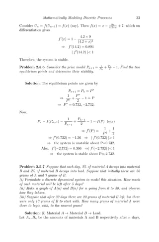
(ii) From Figure 2.9, it is clear that material A slowly decreases, whereas
material B increases till n = 20 and then slowly decreases.
(iii) Here, a = 0.03, b = 0.09, B30 = 20 and B0 = 10
B30 = (1 − 0.09)30
× 10 +
0.03 × A0(0.9730
− 0.9130
)
0.06
= 20
A0 = 113.51 ≈ 114 g.
Problem 2.5.8 Suppose you have a roll of paper, such as paper towels. Let
the radius of the cardboard core be 0.5 inches. Suppose the paper is 0.002 inches
thick. Let r(n) represent the radius, in inches, of the roll when the paper has
been wrapped around the core n times. Let l(n) be the total length of the paper
when it is wrapped about the core n times. Note that r(0)=0.5 and l(0)=0.
Remember, the circumference of a circle is given by c = 2πr.
(i) Develop a dynamical system for r(n) in terms of r(n-1).
(ii) Develop a dynamical system for l(n) in terms of r(n-1) and l(n-1).
(iii) What is the length of paper on the roll when it has a radius of 2 inches?

66. Mathematically Modeling Discrete Processes 35
10 20 30 40 50
Time
50
100
150
200
250
300
Materials
FIGURE 2.9: The behavior of material A(n) and material B(n) with respect
to time in days.
Solution: (i) Let Rn be the radius when paper is wrapped n times and
Ln be the length of paper used for wrapping till n times.
Rn = Rn−1 + t (thickness of paper)
R1 = R0 + t
R2 = R1 + t = R0 + 2t
R3 = R2 + t = R0 + 3t
...... .. ...............................
⇒ Rn = R0 + nt
(ii)
Ln = Ln−1 + 2πRn−1
L1 = L0 + 2πR0 = 2πR0 (∵ L0 = 0)
L2 = L1 + 2πR1 = 2πR0 + 2πR0 + 2πt = 4πR0 + 2πt
L3 = L2 + 2πR2 = 4πR0 + 2πt + 2πR0 + 4πt
L3 = 6πR0 + 6πt
L4 = L3 + 2πR3 = 6πR0 + 6πt + 2πR0 + 6πt
= 8πR0 + 12πt
..... .. ........................................
∴ Ln = 2πnR0 + n(n + 1)πt

67. 36 Mathematical Modeling: Models, Analysis and Applications
(iii) Now, given R0 = 0.5 inches, t = 0.002 inches and L0 = 0, which implies,
Rn = 0.5 + 0.002n and Ln = πn + 0.002πn(n + 1)
We have to find the length of the paper when the radius of the roll is 2 inches,
that is, Rn = 2. Therefore,
2 = 0.5 + 0.002n
⇒ n =
1.5
0.002
= 750. Therefore,
L150 = 2π × 750 × 0.5 + 750 × 751π × 0.002
= 5895.2 inches.
Problem 2.5.9 Presently you weigh 169 pounds. You consume x pounds
worth of calories each week. Assume your body burns off the equivalent of
3% of its weight each week through normal metabolism. In addition, you burn
off 1
4 pound of weight through daily exercise each week. Find x to one decimal
place if you want to weigh between 144 and 146 pounds in 1 year (52 weeks).
Solution: Let Wn be the weight after n weeks. The calories consumed
each week is x pounds and W0 = initial weight = 169 pounds.
Wn = Wn−1 − 0.03Wn−1 − 0.25 + x
Wn = 0.97Wn−1 + x − 0.25
W1 = 0.97W0 + x − 0.25
W2 = 0.97W1 + x − 0.25 = 0.972
W0 + (x − 0.25)[1 + 0.97]
W3 = 0.97W2 + x − 0.25 = 0.973
W0 + (x − 0.25)[1 + 0.97 + 0.972
]
Wn = 0.97n
W0 + (x − 0.25)
[1 − 0.97n
]
1 − 0.97
Now, according to the problem,
144 W52 146
⇒ 144 (0.97)52
× 169 + (x−0.25)
0.03 [1 − (0.97)52
] 146
⇒ 4.375 x 4.45
⇒ x = 4.4 pounds worth of calories.
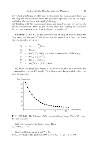
Problem 2.5.10 A certain drug is effective in treating a disease if the con-
centration remains above 100 mg/L. The initial concentration is 640 mg/L. It
is known from laboratory experiments that the drug decays at the rate of 20%
of the amount present each hour.
(i) Formulate a linear discrete system that models the concentration after each
hour.
(ii) Find graphically at what hour the concentration reaches 100 mg/L.
(iii) Modify your model to include a maintenance dose administered every
hour.

68. Mathematically Modeling Discrete Processes 37
(iv) Check graphically or otherwise to determine the maintenance doses that
will keep the concentration above the minimum effective level of 100 mg/L,
and below the maximum safe level of 800 mg/L.
(v) Working with the maintenance doses you found in (iv), try varying the
initial concentration. What do you observe about the tendency to stay within
the necessary bounds, as well as the long-term tendency?
Solution: (i) Let Cn be the concentration of drug at hour n. Since the
drug decays at the rate of 20% of the amount present each hour, the linear
discrete model is given by
Cn = Cn−1 −
20
100
Cn−1
Cn = 0.8Cn−1
C1 = 0.8C0 (C0 being the initial concentration of the drug)
C2 = 0.8C1 = (0.8)2
C0
C3 = 0.8C2 = (0.8)3
C0
∴ Cn = (0.8)n
C0 = (0.8)n
× 640.
(ii) From the graph (see Figure 2.10), we can see that after 9 hours, the
concentration reaches 100 mg/L. Thus, doses must be provided before this
time for recovery.
5 10 15 20
Time in Hours
100
200
300
400
500
600
Drug Concentration
FIGURE 2.10: The behavior of the concentration of drugs C(n) with respect
to time in hours.
(iii) Let x ml/L be the hourly dose. Then,
Cn = 0.8Cn−1 + x
(iv) Equilibrium solution is C∗
= 5x.
Now, according to the problem, 100 5x 800 ⇒ 20 x 160.

69. 38 Mathematical Modeling: Models, Analysis and Applications
5 10 15 20
Time in Hours
200
400
600
800
1000
Drug Concentration
FIGURE 2.11: The effect of different maintenance doses, namely, x =
10, 40, 120, 200 on the concentration of drugs Cn.
The value of the maintenance dose must lie between 20 and 160, which is
clearly understood from the graph (see Figure 2.11).
(v) The final concentration doesn’t depend on the value of the initial dose.
Hence, our bounds remain the same even with change in initial dose (this can
be easily verified from the graph and is left for the reader).
2.6 Exercises
1. Let An be the total value of an investment at the end of n-terms, earning
a compound interest at a rate of r per term, with an additional deposit
of d at the end of each term.
(i) Construct an Annuity Saving Model, assuming A0 to be the original
investment.
(ii) Find the total value after 3 years if the initial investment is Rs. 10000
(Indian Rupees), each month the account gets 1% interest and Rs. 1000
are deposited each month.
(iii) Find the total value after 7 years if the initial investment is Rs.
20000, the account gets 6% annual interest compounded monthly and a
deposit of Rs. 3000 is made each month.
2. Let Ln be the unpaid balance on a loan with an interest rate of r per
term. A payment of P is made at the end of each year.
(i) Assuming L0 to be the original amount borrowed, construct a loan
payment model for the unpaid balance at the end of each n years.
(ii) Find the balance after 3 years when payments of Rs. 500 are made

70. Mathematically Modeling Discrete Processes 39
quarterly on an original loan of Rs. 9600 with an interest rate of 10.5%
per quarter.
(iii) Find the balance after 5 years when a payment of Rupees. 400 is
made monthly on an original loan of Rs. 20000 with annual interest of
8%.
3. Let Pn be the population of the n-th generation, growing linearly at
a rate r and undergoing either immigration or migration at a constant
level k.
(i) Formulate a linear discrete immigration/migration model.
(ii) Find the population of the 4-th generation when the initial popula-
tion is 3900, the growth rate is 7% per generation and immigration is
occurring at a constant rate of 190 per generation.
(iii) Demonstrate the population of the 4-th generation changes if there
is a migration of 190 per generation, instead of immigration.
4. Let Tn be the amount of pollutant present in a contaminated lake, which
is cleaned by filtering out a certain fraction α of all pollutants present at
that time, but another β tons of pollutants seep in (0 α 1, β 0).
(i) Formulate a mathematical model, assuming T0 tons of pollutants are
initially in that lake.
(ii) If each week 10% of all pollutants present can be removed but an-
other 2 tons seep in, find the values of α and β and write the iterate
equation for this process.
(iii) How many tons of pollutant will be in the lake after 2 years if ini-
tially it is contaminated with 70 tons of pollutant?
(iv) How long will it take before the pollutant level falls below 2 tons?
5. Let a pendulum swing in such a manner that the greatest negative (or
positive) angle it makes on one side of the vertical is always a certain
negative fraction (−α) of the greatest positive (or negative) angle it
previously made on the other side of the vertical (0 α 1).
(i) Formulate a mathematical model for this process if θn is the n-th
greatest angle (positive or negative) and θ0 is the initial angle of the
pendulum when released. Hence, write the iterative equation if θ0 =
10 ◦
F and θ2 = 8 ◦
F.
(ii) Suppose the greatest negative (or positive) angle it makes on one
side of the vertical is always 5% of the greatest positive (or negative)
angle it previously made on the other side of the vertical, which always
occurs 3 seconds earlier. How many times will the pendulum cross the
vertical before the magnitude of the angle it achieves is 1 ◦
F or less?
(iii) Approximately how long will it take for this to happen?
6. Suppose a person is saving for retirement by depositing equal amounts
every quarter into a retirement plan to earn 9% annual interest com-
pounded quarterly. If the account initially had zero balance,
(i) How much will be available at retirement time in 25 years if each

71. 40 Mathematical Modeling: Models, Analysis and Applications
deposit is Rs. 10,000.00?
(ii) How much should each deposit be to have Rs. 2,000,000.00 at retire-
ment in 25 years?
7. In a certain forest 3% of the trees are destroyed naturally each year.
Also, 4000 trees are harvested for timber (cut down for industrial use)
but 8000 new trees are either planted or sprout up on their own.
(i) Formulate a discrete model for the yearly number of trees Tn in that
forest.
(ii) What is the maximum number of trees the forest will have in 5 years,
if the currently estimated number of trees in that forest be 200000?
8. A credit card company charges 3% interest on any previous unpaid bal-
ance from a person and the person pays of 20% of that previous balance.
Also, another Rs. 300 is charged on that credit card from the person for
not paying the full amount.
(i) Formulate a discrete model for the monthly unpaid balance.
(ii) What level will the unpaid balance gradually approach?
9. Let a town be affected with viral fever. Each day 10% of those who have
the viral fever in the town recover from it, while another 500 people are
affected with the viral fever. If there are currently 2000 cases of viral
fever,
(i) Formulate a discrete mathematical model and find out how many
cases will be there, two weeks from now.
(ii) At that level, will the number of cases eventually stabilize?
10. It is known that as demand for a product increases, its price increases
and if the price of a product decreases, its supply increases. Let Dn be
the demand, Sn be the supply and Pn be the price of a certain product.
We assume that the demand force increases continuously from negative
to positive as the current demand Dn increases and the same is the
behavior for the supply Sn. Also, as the price of a product increases, its
supply increases but demand from consumers decreases, that is, supply
is directly proportional to the price and demand is inversely proportional
to the price.
(i) Formulate a non-linear discrete price model for the price of a product
at time n from the above information.
(ii) What happens to the above model when the price is close to zero?
How that can be verified by using a different function?
11. Let In be the number of infected population at any given time n and
r be the fraction of the infected population who have recovered in time
(n + 1). It is assumed that the numbers of newly infected population
are directly proportional to the size of the infected population In and to
the size of the susceptible population N −In, where N is the population
size.

72. Mathematically Modeling Discrete Processes 41
(i) Formulate a discrete contagious disease model for the infected pop-
ulation In+1.
(ii) Write down the model when the number of cases is proportional to
(a) I2
n and (1 − In
N )2
, (b) I2
n and (1 −
I2
n
N2 ), (c) In and exp(−In
N )
(iii) In a population of size 106
, each week 80% of those infected recover.
If 1000 are infected in one week, then the following week 1500 are in-
fected. Formulate a mathematical model.
(iv) In a population of size 4 × 106
, 40% infected are still sick after a
week and the maximum number of new infected cases possible in any
week is 50000. Formulate a model with this information.
(v) In a population of size 10000, if 100 are infected, the number doubles
in the following week. Formulate a model for assuming recovery is not
possible.
12. A radioactive element is known to decay at the rate of 2% every 20
years.
(i) If initially you had 165 grams of this element, how much would you
have in 60 years?
(ii) What is the half-life of this element?
(iii) Suppose that the bones of a certain animal maintains a constant
level of this element while the animal is living, but the element begins
to decay as soon as the animal dies. If a bone of this animal is found
and is determined to have only 10% of its original level of this element,
how old is the bone?
13. A population of weasels is growing at the rate of 3% per year. Let wn
be the number of weasels, n years from now and suppose that there are
currently 350 weasels.
(i) Formulate a linear discrete model which describes how the population
changes from year to year.
(ii) Solve the difference equation of part (i). If the population growth
continues at the rate of 3%, how many weasels will there be 15 years
from now?
(iii) Plot wn versus n for n = 0, 1, 2, ..., 100.
(iv) How many years will it take for the population to double?
(v) Find limn→∞wn. What does this say about the long-term size of the
population? Will this really happen?
(vi) If the rate of growth of the weasel population was 5% instead of 3%,
how many years would it take for the population to double?
14. A cup of coffee has an initial temperature of 165 ◦
F, but cools to 155 ◦
F
in one minute when placed in a room with a temperature of 70 ◦
F. Let
Tn be the temperature of the coffee after n minutes.
(i) Formulate a linear discrete model which describes the change in tem-
perature of the coffee from minute to minute and solve it.
(ii) Find the temperature of the coffee after 25 minutes.

73. 42 Mathematical Modeling: Models, Analysis and Applications
(iii) Find limn→∞Tn.
(iv) Plot Tn versus n for n = 0, 1, 2, ...120.
(v) Does the temperature ever reach 70 ◦
F?
15. The forensics team from a local police department is called to the scene
of an apparent murder. The body of the victim is found in a room where
the thermostat was set at 72 ◦
F. The police investigators believe that the
victim died in the room and that the body has been there ever since.
(i) Formulate a linear discrete system that describes how the tempera-
ture of the dead body changes from hour to hour and solve it.
(ii) At 5 A.M., when the investigators first arrived, they took the tem-
perature of the body and found that it was 87.5 ◦
F. Just before the body
was to be removed from the room an hour later, they measured the tem-
perature to be 80.4 ◦
F. Find the time when the victim was murdered.
(iii) Using the data from (ii), modify the difference equation to describe
how the temperature of the dead body changes
(a) over each 15-minute interval
(b) from minute to minute.
16. An industry dumps a metal-based pollutant into a local lake. Currently
there are 350 pounds of pollutant in the lake and 20 pounds are added
each year, all at once at the end of the year. It is known that the amount
of pollutant lost through evaporation and decomposed chemically in a
year is 10% of the amount in the lake.
(i) Formulate a linear discrete system that models the amount of the
pollutant in the lake after each year.
(ii) Show graphically, what will happen in the long run if the situation
described above persists. How does the outcome depend on the initial
amount of the pollutant in the lake?
(iii) The maximum safe amount of pollutant in this lake is 125 pounds of
pollutant. If we set a goal to achieve this safe level in 15 years, determine
how much pollutant can be added to the lake each year.
(iv) What, if the amount of pollutant that is added each year is divided
into equal parcels, are added each month throughout the year? How does
this change the model in part (i) and the results obtained in parts (ii)
and (iii)?
17. A person has signed a contract to write a book, where he has already
written the first 90 pages. But, the publisher wants the book to be 300
pages long. The author has started writing K pages of the book, each
day, starting from today.
(i) Formulate a linear discrete system that models wn, the total number
of pages written after n days and the unknown parameter K, taking
w(0) = 90.
(ii) The publisher has given the author 21 days to finish the book. Find

74. Mathematically Modeling Discrete Processes 43
the approximate number of pages the author needs to write each day to
complete the book.
18. You are counseling a recent graduate on retirement planning. You es-
timate he will earn 9% per year (or 0.75% per month) on a retirement
account. With his high-paying job, he will be able to invest Rupees 5000
per month initially. To allow for inflation and pay raises, you suggest
increasing this amount by 0.5% per month. Assume that he makes his
first deposit at the end of his first month of employment.
(i) Formulate a discrete dynamical system that models the amount in
this person’s retirement account and solve it.
(ii) Graphically, determine the balance in the account after 20 years and
use the analytic solution to verify it.
(iii) How does the analytic solution change if the monthly investment
increases by 0.75% per month instead of 0.5% per month?
19. Let the kidneys filter out 45% of the vitamin A in the plasma each day
and the liver absorb 35% of the vitamin A in the plasma each day. Also,
2% of the vitamin A in the liver is absorbed back into the plasma each
day. Let 15% of the vitamin A in the plasma convert to a chemical B
and 5% of the chemical B is filtered out by the kidney each day. Assume
that the daily intake is 2 mg of vitamin A and 1 mg of the chemical B
each day.
(i) Formulate a discrete dynamical model for vitamin A in the plasma,
vitamin A in the liver and chemical B.
(ii) Find the equilibrium solution and check for its stability.
(iii) Suppose a person ingests 1.4 mg of vitamin A each day and wants
the equilibrium for vitamin A in the plasma to be 3 mg. How much of
the chemical B should you ingest each day to accomplish this? What
will be the equilibrium amount of the chemical B in the plasma and
what will be the equilibrium amount of vitamin A in the liver with this
consumption?
20. Consider a linear predator-prey model. Let the prey’s growth rate be
1.2 and that of the predator be 1.3; the prey population diminishes by
0.3 times that of the predator; the predator’s population is increased by
0.4 times that of the prey. Construct a discrete model from the given
information and discuss its stability.
21. Let the two species xn and yn compete for food, water, habitat etc. at
any time n. Both the species grow at the rate r1 and r2 respectively
and they diminish by an amount directly proportional to the size of the
other, say at a rate S1 and S2 respectively.
(i) Formulate a linear competition model with the above information.
(ii) Suppose there is a constant migration or constant immigration, K1
and K2 respectively, how will the model change?

75. 44 Mathematical Modeling: Models, Analysis and Applications
(iii) Let the growth rate r1 of the first species be 1.5 and that of the sec-
ond species be 1.25. Also, each is diminished by 0.4 times the population
of the other. Construct a discrete model and comment on its stability.
(iv) In addition to the information in (iii), if the first species undergoes
immigration of 2500 at each time step and the second one migrates at
1200 per time step, formulate a new model and comment on its stability.
22. A soccer player gets a contract for Rs. 50000.00 (Indian Rupees) per
game and a Rs. 3,00,000.00 signing bonus.
(i) Formulate a discrete dynamical system to model this player’s earnings
over the season.
(ii) How much will this player earn if he plays 120 games and how many
games does he need to play to earn at least Rs. 1,000,000?
23. A car holds 30 litres of petrol (full tank) and gets 10 km to a litre of
petrol.
(i) Formulate a discrete dynamical system to model the amount of petrol
left in the car’s tank after driving for x km.
(ii) How much gas will be left in the tank after you have driven 120 km
and how many km can you drive before running out of petrol?
24. Research evidence has shown that the number of chirps some crickets
make depends on the temperature. At 70 ◦
F, one species of cricket makes
about 124 chirps per minute. The number of chirps increases by 4 per
minute for each degree the temperature rises. Formulate a discrete dy-
namical system to model the situation that relates the number of chirps
per minute in terms of the temperature and use this expression to find
the approximate temperature if you count about 24 chirps in 10 seconds.
25. The pavement on a bridge is 1000 m long at 70 ◦
F. The length of the
pavement grows by 0.012 m for each degree rise in temperature. Formu-
late a discrete dynamical system to model the length of the bridge in
terms of the temperature. What will be the length of the bridge if the
temperature reaches 105 ◦
F?
26. The air pressure at sea level is 1000 g/cm2
. The pressure increases by
2.08 g/cm2
for each cm of depth in salt water. Write a discrete mathe-
matical model for this discrete dynamical system.
27. Most of us keep the water tap open while shaving. In this problem, we
are going to study how water is wasted during shaving. Let w(n) be the
amount of water that is wasted per day by n number of people that let
the water run while shaving.

76. Mathematically Modeling Discrete Processes 45
(i) Formulate a discrete dynamical system to model this situation.
(ii) Assuming you shave 5 times a week, estimate how much water would
be wasted per day if you leave the water running while shaving.
28. Each year, a person who smokes a single pack of cigarettes a day will
absorb about 2.7 mg of cadmium (an extremely dangerous heavy-metal
pollutant that is most toxic when inhaled). For simplicity it is assumed
that the cadmium is absorbed at the end of the year. Some people elim-
inate about 8% of the cadmium from their bodies each year. Formulate
a dynamical system for u(n), the amount of cadmium in such a person’s
body after n years as a result of smoking and hence find the amount of
cadmium in such a person’s body as a result of smoking for 20 years.
29. A boy absorbs 0.4 mg of lead into his plasma each day, starting from to-
day. Each day, 35% of the lead in his plasma is absorbed into his bones
and 9% of the lead in his plasma is eliminated in the urine (approx-
imately). Also, 0.118% of the lead in his bones is absorbed back into
his plasma each day. Formulate a discrete mathematical model for this
situation, assuming p(n) to be the amount of lead in this boy’s plasma
and b(n) to be the amount of lead in this boy’s bones, at the beginning
of day n. Hence, find p(4) and b(4), where p(0)=0 and b(0)=0.
30. Suppose a person’s body burns 130 kcal per week for each pound it
weighs. Suppose this person presently weighs 165 pounds and consumes
about 21,000 kcal per week. Suppose this person decides to eat 200 kcal
less each week than the week before. Let c(n) represent the number of
kilocalories this person consumes during the n-th week of this diet and
w(n) be the weight of this person after n weeks of this diet. Develop
a dynamical system of two equations, one for c(n) and one for w(n),
assuming c(1)=20,800 and w(0)=165 (to work this problem, you need to
know that burning 3600 kcal would reduce a person’s weight by 1 pound
and consuming 3600 kcal would result in the gaining of 1 pound).

78. Chapter 3
Continuous Models Using Ordinary
Differential Equations
3.1 Introduction to Continuous Models ....................................... 47
3.2 Formation of Various Continuous Models ................................ 48
3.2.1 Carbon Dating .................................................... 48
3.2.2 Drug Distribution in the Body .................................... 49
3.2.3 Growth and Decay of Current in an L-R Circuit ................. 50
3.2.4 Rectilinear Motion under Variable Force ......................... 52
3.2.5 Mechanical Oscillations ........................................... 53
3.2.5.1 Horizontal Oscillations ................................... 53
3.2.5.2 Vertical Oscillations ..................................... 54
3.2.5.3 Damped Force Oscillation ............................... 55
3.2.6 Dynamics of Rowing .............................................. 57
3.2.7 Arms Race Models ................................................ 58
3.2.8 Mathematical Model of Influenza Infection (within Host) ........ 60
3.2.9 Epidemic Models .................................................. 61
3.3 Steady State Solutions .................................................... 65
3.4 Linearization and Local Stability Analysis ............................... 66
3.5 Phase Plane Diagrams of Linear Systems ................................ 68
3.6 Bifurcations ............................................................... 72
3.6.1 Saddle-Node Bifurcation .......................................... 73
3.6.2 Transcritical Bifurcation .......................................... 75
3.6.3 Pitchfork Bifurcation .............................................. 77
3.6.4 Hopf Bifurcation .................................................. 79
3.7 Miscellaneous Examples ................................................... 80
3.8 Exercises .................................................................. 98
3.1 Introduction to Continuous Models
Continuous models are systems whose inputs and outputs are capable of
changing at any instant of time. A continuous model consists of a dependent
continuous variable, varying with some other independent continuous vari-
ables. We use a first order ordinary differential equation (or a system of first
order ordinary differential equations) to model a continuous system, if we have
some information or assumption about the rate of change of the dependent
variable(s) with respect to the independent variable(s). The continuous sys-
tem is modeled with a partial differential equation, if the dependent variable
depends on more than one independent variables.
47

79. 48 Mathematical Modeling: Models, Analysis and Applications
3.2 Formation of Various Continuous Models
3.2.1 Carbon Dating
Carbon dating (Carbon 14 dating) is a method, developed by W.F. Libby
at the University of Chicago in 1947 [76], that can be used to accurately
date archaeological samples to determine the ages of plant (wood fossil) or
any material which got its carbon from air. Carbon 14 (C14
), a radioactive
isotope of carbon, is a result of constant bombardment by radiation from the
sun in the atmosphere. During this bombardment, neutrons hit nitrogen 14
atoms and transmute them to carbon.
In a living organism, the absorption rate of C14
balances the disintegration
rate of C14
. When the organism dies and the body is preserved, it does not
absorb C14
but disintegration continues. As mentioned before, C14
is radioac-
tive in nature and has a half-life (the time taken by a substance undergoing
decay to decrease to half) of 5730 years. Scientists use this information. The
method of carbon dating involves measuring the strength of C14
archaeolog-
ical samples or fossils and then comparing it with the expected strength of
C14
in the atmosphere, to calculate the accurate age.
Suppose an archaeological sample was found whose age needs to be deter-
mined. Let A(t) be the amount of C14
present in the sample at any time t,
then
dA
dt
= −λA (following radioactive decay law) (3.1)
where λ is the decay constant of the sample.
Integrating, we get,
A(t) = A0e−λt
,
where A0 = A(0) is the amount of C14
present in the sample when it was dis-
covered. From equation (3.1), we can obtain the present ratio of disintegration
of C14
in the archaeological sample, given by
M(t) = −
dA
dt
= λA0e−λt
⇒
M(t)
M(0)
= e−λt
, M(0) = λA0,
being the original rate of disintegration.
⇒ t =
1
λ
log
M(0)
M(t)
. (3.2)
From (3.2), we can determine the age, provided we can measure M(t) and
M(0). M(0) should be equal to the rate of disintegration of C14
in a compa-
rable amount of archaeological sample or fossil (living wood).

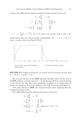
80. Continuous Models Using Ordinary Differential Equations 49
The half-life of the sample under investigation can be obtained from equa-
tion (3.2). Since the half-life is the amount of time required by the decreasing
substance to reduce to half, we get
A0
2
= A0e−λτ
, where τ is the half-life.
τ =
1
λ
loge 2 =
0.6931
λ
.
3.2.2 Drug Distribution in the Body
The study of movement of drug in the body is called pharmacokinetics. The
science of pharmacokinetics uses mathematical equations and utilizes them to
describe the movement of the drug through the body [54].
We now study a simple problem in pharmacology, where we will be dealing
with the dose-response relationship of a drug. In this problem, the drug present
in the system follows certain laws. Let us assume that the rate of decrease of
the concentration of the drug is directly proportional to the square of its
amount present in the body and C0 be the initial dose of the drug given to
the patient at time t = 0. The mathematical model that captures this dynamic
is given by
dC(t)
dt
= −kC2
(3.3)
where k is a constant depending on the drug used, and its value can be ob-
tained from experiment. Solving (3.3), we get
⇒ C(t) =
C0
1 + C0kt
, where C(0) = C0.
Let an equal dose of drug C0 be given to the body at equal time intervals, T .
Then, immediately after the second dose, the concentration of the drug inside
the body is
C1 = C0 +
C0
1 + C0kT
Immediately after the third dose, the concentration of the drug inside the
body is
C2 = C0 +
C1
1 + C1kT
In a similar manner, we can conclude that
Cn = C0 +
Cn−1
1 + Cn−1kT
, (3.4)
which is a non-linear difference equation. Now,
Cn+1 − Cn =
Cn − Cn−1
(1 + kT Cn)(1 + kT Cn−1)
, (3.5)

81. 50 Mathematical Modeling: Models, Analysis and Applications
From (3.4), we conclude that Cn C0, which implies Cn+1−Cn and Cn−Cn−1
have the same sign. Noting that Cn is an increasing function of n, we attempt
to find the limiting value of the concentration by taking limits on both sides
of (3.4), that is,
lim
t→∞
Cn = lim
t→∞
C0 +
Cn−1
1 + Cn−1kT
⇒ lim
t→∞
Cn = C0 +
limt→∞ Cn−1
1 + kT limt→∞ Cn−1
C∞ = C0 +
C∞
1 + C∞kT
where C∞ = lim
t→∞
Cn = lim
t→∞
Cn−1
kT C2
∞ − kT C0C∞ − C0 = 0
C∞ =
kT C0 ±
k2T 2C2
0 + 4C0kT
2kT
C∞ =
C0
2
+
C0
2
1 +
4
C0kT
(taking positive signs only).
This implies C0 Cn C∞, that is, the concentration is bounded.
3.2.3 Growth and Decay of Current in an L-R Circuit
FIGURE 3.1: The inductance-resistance (L-R) circuit, connected to a battery
of voltage V through a key K.
We consider an L-R circuit where L is the inductance of the coil and R is
the resistance. The coil is connected to a battery of voltage V through a key
K (Figure 3.1).
In the ON position, the current flows through the coil. When the current
i(t) starts to flow, the negative lines of force move outward from the coil and
an electromotive force (e.m.f.) will induce across L. According to the law of
electromagnetic induction, this e.m.f. will oppose the voltage, as a result of
which there will be a voltage drop across R, which will also oppose the applied

82. Continuous Models Using Ordinary Differential Equations 51
voltage. The differential equation modeling of this scenario is given by
V − L
di
dt
= Ri
⇒
i
0
di
i − V
R
= −
R
L
t
0
dt
⇒ loge
i −
i
V/R
= −
R
L
t
⇒ i =
V
R
1 − e− R
L t
(at t = 0, there is no current, that is, i(0) = 0)
which shows that the current grows exponentially. As t → ∞, i → V
R = I
(say), a steady value (see Figure 3.2(a)).
100 200 300 400 500
10
20
30
40
50
(a) Current grows and reaches a
steady value.
100 200 300 400 500
10
20
30
40
50
(b) Current decays to zero.
FIGURE 3.2: Graphs showing the (a) growth and (b) decay of current, with
L = 50, R = 1 and V = 50.
We now put the key in the OFF position. Initially, when the key was in
the ON position, a steady current I = V
R was flowing. With no current flowing
in the circuit, the flux will reduce gradually, resulting in a voltage drop iR
across the resistance R and the induced e.m.f. Ldi
dt across the inductance L.
Now, since the key is OFF, the current becomes open, implying that the
impressed voltage is zero.
The differential equation showing this decay is given by
0 − L
di
dt
= iR
⇒
i
I
di
i
= −
t
0
R
L
dt
log
i
I
= −
R
L
t (Since at t = 0, i = I)
⇒ i(t) =
V
R
e− R
L t

83. 52 Mathematical Modeling: Models, Analysis and Applications
Thus, the current decays exponentially as time increases and ultimately goes
to zero (see Figure 3.2(b)).
3.2.4 Rectilinear Motion under Variable Force
FIGURE 3.3: A particle moving in a straight line towards the origin O
(fixed) and acted upon by a force P.
Let a particle move in a straight line and be acted upon by a force P = mμ
x ,
μ( 0) being the constant of proportionality, which is always directed towards
a fixed point O. m is the mass of the particle and x is the distance of the
particle from the fixed point O (Figure 3.3). The equation of motion modeling
the given scenario is given by
mv
dv
dx
= −m
μ
x
, where v
dv
dx
is the acceleration of the particle of mass m.
Since the force is attractive, the sign of right hand side is negative. Integrating,
we get,
v2
2
= −μlogex + Constant
Initially, let the particle start from rest at a distance a from the fixed point
O (origin), then at the time t = 0, x = a, v = 0
⇒ Constant = μlogea
⇒ v2
= 2μloge
a
x
⇒ v =
dx
dt
= −
2μloge
a
x
(negative sign as distance decreases with time)
⇒
2μ
T
0
dt = −
0
a
dx
loge
a
x

84. Continuous Models Using Ordinary Differential Equations 53
where T is the time the particle takes to reach the origin.
∴
2μT = −
∞
0
ae−y2
(−2y)dy
y
take loge
a
x
= y2
= 2a
∞
0
e−y2
dy = 2a
√
π
2
⇒ T = a
π
2μ
.
3.2.5 Mechanical Oscillations
3.2.5.1 Horizontal Oscillations
FIGURE 3.4: A particle at rest is attracted by two forces towards two fixed
centers O1 and O2 respectively.
We consider a particle of mass m resting in equilibrium at a point A, being
attracted by two forces equal to mμn
1 × (distance)n
and mμn
2 × (distance)n
respectively, towards two fixed centers O1 and O2 (Figure 3.4).
In this equilibrium position of the particle at A, the forces acting on it are
equal and opposite and hence O1, A and O2 are collinear.
Let O1O2 = a, O1A = d1 and AO2 = d2. Then d1 + d2 = a and μn
1 dn
1 =
μn
2 dn
2 , since the forces are equal and opposite at A.
μ1d1 = μ2d2
⇒
μ1
d2
=
μ2
d1
=
μ1 + μ2
d1 + d2
=
μ1 + μ2
a
⇒ d1 =
aμ2
μ1 + μ2
and d2 =
aμ1
μ1 + μ2
Now, let the particle be slightly displaced towards the fixed center O2 and P
be the new position of the particle at any time t, such that AP = x (small).
The differential equation modeling of this physical scenario is given by
m
d2
x
dt2
= −mμn
1 O1Pn
+ mμn
2 O2Pn
(3.6)
When the particle is slightly displaced from the equilibrium position A to
the position P, it tends to come back to its original position. Doing so, O1

85. 54 Mathematical Modeling: Models, Analysis and Applications
becomes the point of attraction and O2 the origin of repulsion. This explains
the first term on the right hand side of (3.6) to be negative and the second
term to be positive.
∴
d2
x
dt2
= −μn
1 (d1 + x)n
+ μn
2 (d2 − x)n
= −μn
1 dn
1
1 +
x
d1
n
+ μn
2 dn
2
1 −
x
d2
n
= −μn
1 dn
1
1 +
nx
d1
+
n(n − 1)
2!
x2
d2
1
+ ...
+ μn
2 dn
2
1 −
nx
d2
+
n(n − 1)
2!
x2
d2
2
+ ...
or,
d2
x
dt2
= −μn
1 dn
1 − nxμn
1 dn−1
1 + μn
2 dn
2 − nxμn
2 dn−1
2
(Since x is small, neglecting higher powers of x)
⇒
d2
x
dt2
= −n
μn
1 dn−1
1 + μn
2 dn−1
2
x
= −n
μn
1
aμ2
μ1 + μ2
n−1
+ μn
2
aμ1
μ1 + μ2
n−1
x
= −
nμn−1
1 μn−1
2 an−1
(μ1 + μ2)n−1
(μ1 + μ2)x
or,
d2
x
dt2
= −n
(μ1μ2a)n−1
(μ1 + μ2)n−2
x
Therefore, we conclude that the motion of the particle is simple harmonic
about A and the period of oscillation is
2π
(μ1 + μ2)n−2
(μ1μ2a)n−1
.
3.2.5.2 Vertical Oscillations
Consider an elastic string of upstretched length AB(= a), fixed at point A.
A particle of mass m is attached to the end of the string, so that the string is
extended to the length AO(= b) when the mass is at rest. In the equilibrium
position, the tension in the string is balanced by the weight of the particle,
that is,
mg = T0 = λ
AO − AB
AB
(by Hooke’s law)
⇒ mg = λ
b − a
a
, λ is the modulus of elasticity. (3.7)

86. Continuous Models Using Ordinary Differential Equations 55
FIGURE 3.5: A vertical elastic string AB is pulled to the point D and let
go.
Now, the particle is pulled to the point D and let go. Let P be the position
of the particle at any time t such that OP = x (see Figure 3.5).
The differential equation that models the scenario is given by
m
d2
x
dt2
= mg − T, where T is the tension of the string.
⇒ m
d2
x
dt2
= mg − λ
b + x − a
a
= mg − λ
b − a
a
−
λx
a
⇒
d2
x
dt2
= −
λx
am
(using (3.7))
Hence, the motion is simple harmonic about the center O, the period of oscil-
lation being 2π
am
λ .
3.2.5.3 Damped Force Oscillation
FIGURE 3.6: A disturbing force 2kv acting on a particle moving in a straight
line towards a fixed point O.
We consider a particle moving in a straight line with an acceleration μ2
(distance) towards a fixed point O in the line. A disturbing acceleration 2k

87. 56 Mathematical Modeling: Models, Analysis and Applications
(velocity)(μ k) also acts on the particle along with a periodic additional
acceleration F cos(bt) [49] (see Figure 3.6).
The equation of motion that models the scenario is given by
d2
x
dt2
= −μ2
x − 2k
dx
dt
+ F cos(bt).
Let x = Aemt
(A = 0) be a trial solution of
d2
x
dt2
+ 2k
dx
dt
+ μ2
x = 0,
then the required auxiliary equation is
m2
+ 2mk + μ2
= 0 ⇒ m = −k ±
k2 − μ2
= −k ± i
μ2 − k2 (μ k)
Complimentary function is e−kt
A cos(
μ2 − k2t + ε1) and the particular in-
tegral is given by
1
D2 + 2Dk + μ2
F cos(bt) = F
D2
− 2Dk + μ2
(D2 + μ2)2 − 4D2k2
cos(bt)
= F
(μ2
− b2
) cos(bt) + 2kb sin(bt)
(μ2 − b2)2 + 4k2b2
= B cos(bt − ε2)
where B =
F
(μ2 − b2)2 + 4k2b2
and tan ε2 =
2kb
μ2 − b2
Therefore, the general solution is
x = Ae−kt
cos(
μ2 − k2t + ε1) + B cos(bt − ε2) (3.8)
From (3.8), it is concluded that motion is the resultant of two oscillations,
namely, the free oscillation (first part) and forced oscillation (second part).
The arbitrary constants A and B can be obtained from the initial conditions.
From the expression (3.8), it is clear that the amplitude of free oscillation
decreases with time t because of the factor e−kt
and ultimately vanishes for
large t. However, the amplitude of the forced oscillation persists as there is no
diminishing factor, whose period of oscillation is 2π
b . This is also evident from
Figure 3.7.
Special Case: If the period of forced oscillation is equal to the period
of free oscillation, that is, 2π
b = 2π
μ ⇒ b = μ, then the amplitude of the
forced oscillation is B = F
2kb . If k is small, then the amplitude of the forced
oscillation is very large. This is the reason why a group of soldiers marching
on a bridge are ordered to fall out. While marching in groups, the period of
forced vibration may be equal to the natural period of the bridge structure.
Then a large amplitude of vibration may be generated, which may cause the
bridge to crack and fall down.

88. Continuous Models Using Ordinary Differential Equations 57
50 100 150 200 250
0.5
0.5
1.0
FIGURE 3.7: A motion which is the resultant of two oscillations, namely,
a free oscillation and a forced one.
3.2.6 Dynamics of Rowing
In rowing a boat, a person tries to push the boat forward against the water
using the oar and thereby exerts a force, known as tractive force. We denote
that force by T . Also, as the boat moves forward, the water adjacent to the
sides of the boat exerts a force, resulting in losing its speed. We call this force
a drag force and denote it by D. If v(t) be the velocity of the boat at any time
t, then the equation of motion is given by [53]
M
dv
dt
= T − D
Let us now assume that the person has entered a race and let P be the effective
power that the person can sustain for the entire length he has to row. Then,
from physics, we get
P = T × v (effective power = Tractive force × velocity)
Also, from fluid dynamics, the drag force is proportional to the square of the
velocity and to the surface area in contact with the water (wetted surface
area). Thus,
D = kv2
S
where S is wetted surface area and k is the constant of proportionality. Thus,
the model showing the dynamics of rowing is given by [53]
M
dv
dt
=
P
v
− kv2
S
=
P − kv3
S
v
=
ks( P
kS − v3
)
v

89. 58 Mathematical Modeling: Models, Analysis and Applications
∴
vdv
a3 − v3
=
kS
M
dt where a3
=
P
kS
⇒ log
a2
+ av + v2
(a − v)2
− 2
√
3 tan−1
a + 2v
√
3a
=
6akS
M
t + Constant
Assuming at t = 0, v = 0, we get Constant = − π
√
3
∴ log
a2
+ av + v2
(a − v)2
+
π
√
3
− 2
√
3 tan−1
a + 2v
√
3a
=
6akS
M
t
where a =
P
kS
1/3
. This is more or less what we observe in the race, except
the person rowing the boat may slow down at the end.
3.2.7 Arms Race Models
We consider two neighboring countries A and B and let x(t) and y(t) be the
expenditures on arms respectively by these two countries in some standardized
monetary unit.
We construct a simple mathematical model by assuming the notion of
mutual fear, that is, the more one country spends on arms, it encourages
the other one to increase its expenditure on arms. Thus, we assume that each
country spends on arms at a rate which is directly proportional to the existing
expenditure of the other nation.
Mathematically we can write [93]
dx
dt
= αy (α, β 0)
dy
dt
= βx (3.9)
⇒
d2
x
dt2
= α
dy
dt
= αβx
⇒ x = A1e
√
αβt
+ A2e−
√
αβt
Similarly,
y = B1e
√
αβt
+ B2e−
√
αβt
Thus, x, y → ∞ as t → ∞ and we conclude that both the countries A and
B spend more and more money on arms with increasing time and no lim-
its on the expenditure. As the mathematical prediction of indefinitely large
expenditure for both the countries is unrealistic, an improved model is desired.
In the modified model, other than the mutual fear, we also assume that
the excessive expenditure on the arms puts the country’s economy in the com-
promising position and hence the rate of change of one country’s expenditure

90. Continuous Models Using Ordinary Differential Equations 59
on arms will also be directly proportional to its own expenditure. Model (3.9)
is modified as [93]
dx
dt
= αy − γx (α, β, γ, δ 0)
dy
dt
= βx − δy (3.10)
Clearly, (0, 0) is the only steady state solution, provided γδ − αβ = 0.
The characteristic equation is given by

94. −γ − λ γ
β −δ − λ

98. = 0
⇒ λ2
− (−δ − γ)λ + γδ − αβ = 0.
Hence, the system is stable if γδ − αβ 0.
γδ αβ
This implies if the product of the rates of depreciation (γδ) on the expenditure
of arms of both the countries A and B is greater than the product of rates
of expenditure (αβ) on arms of both the countries, the system will be stable
and the countries will spend an allocated amount of money on arms, so that
the economy of the country is not compromised.
A simplified refinement of model (3.10) was made by Lewis F. Richard-
son (1881-1953), popularly known as the Richardson Arms Race model [104],
where he assumed that the cause of the rate of increase of a country’s ar-
mament, not only depend on mutual stimulation but also on the permanent
underlying grievances of each country against the other. The refined model is
[93, 102, 104]
dx
dt
= αy − γx + r (3.11)
dy
dt
= βx − δy + s (3.12)
where α, β, γ, δ are positive (as before) and r, s are constants which may have
any sign.
The unique steady state solution is given by
αy∗
− γx∗
+ r = 0
βx∗
− δy∗
+ s = 0,
provided γδ − αβ = 0 where
x∗
=
rδ + sα
γδ − αβ
and y∗
=
rβ + sγ
γδ − αβ

99. 60 Mathematical Modeling: Models, Analysis and Applications
The characteristic equation is
λ2
− (−γ − δ)λ + γδ − αβ = 0.
Case I γδ − αβ 0, r 0, s 0. In this case, the system is stable. This
means both the countries spent on arms in a strategic manner so that the
economy of the country is not compromised.
Case II γδ − αβ 0, r 0, s 0. In this case, though the system
is stable, the equilibrium solution becomes negative. However, expenditures
cannot be negative in reality. Suppose (x0, y0) 0 be the initial expenditures,
then x(t) → x∗
and y(t) → y∗
at t → ∞ and for that it has to pass through
zero values. Thus, as x(t) becomes zero, (3.12) reduces to
dy
dt
= −δy + s
⇒ y(t) =
δ
s
+ C1e−δt
Since s 0, y(t) decreases till it reaches the value zero. A similar argument
is valid for x(t). Thus, in this case, both the countries will stop spending on
arms and then this will result in a complete disarmament [63].
Case III γδ − αβ 0, r 0, s 0. In this case, one of the countries has
overcome the grievance (s 0). The system is stable with positive equilibrium
solution if δr + αs 0 and βr + γs 0(s 0). The system approaches
an equilibrium value which is less than the previous cases when both r, s
0. That means when one country has overcome the grievance and started
spending less on armaments, this will have an effect on the other country,
who will also start spending less in order to develop mutual goodwill [63].
Case IV γδ − αβ 0, r 0, s 0. The system becomes unstable, which
will lead to a runaway arms race (x → ∞, y → ∞) as one of the eigenvalues
is positive and the other is negative.
Case V γδ −αβ 0, r 0, s 0. The system is unstable but equilibrium
solution is positive. Though one of the eigenvalues is positive and the other
is negative, there is a possibility of disarmament as well as a runaway arms
race, depending on the initial expenditure on arms by both the countries [63].
3.2.8 Mathematical Model of Influenza Infection (within
Host)
An influenza A infection has the propensity to cause occasional pandame-
cis with potentially high death tolls. Initial infection affects only the upper
respiratory tract and the upper divisions of bronchi. However, in a severe case,
the infection will spread to the lower lungs. A basic mathematical model to

100. Continuous Models Using Ordinary Differential Equations 61
capture the dynamics of influenza A virus within a host is given by [13]
dT
dt
= −βT V
dI
dt
= βT V − δI
dV
dt
= pI − cV
where T is the target cells (namely, epithelial cells of the respiratory tract),
I is the infected cells and V is the influenza A virus. The target cells are
infected by virus, which immediately start producing virions (virus particles)
at a rate β. The infected cells die at a rate δ (by apoptosis). The infected
cells I producing virions undergo a natural death at the rate c. Let the newly
infected cells undergo a latent stage E before they become infectious. In that
case, the modified model will be
dT
dt
= −βT V
dE
dt
= βT V − kE
dI
dt
= kE − δI
dV
dt
= pI − cV
3.2.9 Epidemic Models
In this section, I have discussed various epidemic models where emphasis
has been put on modeling. Mathematical epidemiology is the use of mathe-
matical models to predict the course of an infectious disease and to compare
the effects of differential control strategies.
In epidemic models, the population is divided into three main classes,
namely, a susceptible class, denoted by S(t) (persons who are vulnerable to
the disease or who can be easily infected by the disease), infected class denoted
by I(t) (persons who already have the disease), and recovered class, denoted
by R(t) (persons who have recovered from the disease). One can define more
classes, if the situation demands, for modifications in the models.
Susceptible-Infective Model: Let a population consist of (n+1) persons
of which n persons are susceptibles and only one is infected, so that S(t) +
I(t) = n + 1, S(0) = n, I(0) = 1. A susceptible person gets infected when he
comes in contact with an infected one and mathematically we can say that
the rate of increase of the infected class is proportional to the product of the
susceptible and infected persons. Hence, the susceptible class also decreases

101. 62 Mathematical Modeling: Models, Analysis and Applications
at the same rate. The system of differential equations governing this model is
[63]
dS
dt
= −αSI
dI
dt
= αSI (α 0)
⇒
dS
dt
= −αS(n + 1 − S)
dI
dt
= αI(n + 1 − I)
Integrating and using the initial condition we get,
S(t) =
n(n + 1)
n + e(n+1)βt
and I(t) =
(n + 1)
ne−(n+1)βt + 1
at t → ∞, S(t) → 0 and I(t) → n + 1.
Therefore, we conclude that as time increases, all the susceptible persons
will become infected.
Susceptible-Infective-Susceptible Model: A simple refinement of the
previous model has been made and named as the SIS model where it is as-
sumed that the infected person has the ability to recover and move to the
susceptible class at a rate β (say). Then, we get the SIS model as [63]
dS
dt
= −αSI + βI
dI
dt
= αSI − βI
Since S(t) + I(t) = n + 1, we get
dS
dt
= {α(n + 1) − β}I − αI2
dI
dt
= β(n + 1) − {β + α(n + 1)}S + αS2
Integrating we get
S(t) =
−eβtc1
(1 + n) + e(1+n)α(t+c1)
β
−eβtc1 (1 + n) + e(1+n)α(t+c1)α
I(t) =
(α + nα − β)e(1+n)tα+βc2
−etβ+(1+n)αc1 + e(1+n)tα+βc2 α
where c1 and c2 are arbitrary constants of integration. As t → ∞, S(t) → β/α
and I(t) = 1 + n − β
α , provided (1 + n)α − β 0. Hence, in this case, a

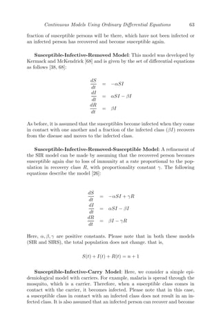
102. Continuous Models Using Ordinary Differential Equations 63
fraction of susceptible persons will be there, which have not been infected or
an infected person has recovered and become susceptible again.
Susceptible-Infective-Removed Model: This model was developed by
Kermack and McKendrick [68] and is given by the set of differential equations
as follows [38, 68]:
dS
dt
= −αSI
dI
dt
= αSI − βI
dR
dt
= βI
As before, it is assumed that the susceptibles become infected when they come
in contact with one another and a fraction of the infected class (βI) recovers
from the disease and moves to the infected class.
Susceptible-Infective-Removed-Susceptible Model: A refinement of
the SIR model can be made by assuming that the recovered person becomes
susceptible again due to loss of immunity at a rate proportional to the pop-
ulation in recovery class R, with proportionality constant γ. The following
equations describe the model [26]:
dS
dt
= −αSI + γR
dI
dt
= αSI − βI
dR
dt
= βI − γR
Here, α, β, γ are positive constants. Please note that in both these models
(SIR and SIRS), the total population does not change. that is,
S(t) + I(t) + R(t) = n + 1
Susceptible-Infective-Carry Model: Here, we consider a simple epi-
demiological model with carriers. For example, malaria is spread through the
mosquito, which is a carrier. Therefore, when a susceptible class comes in
contact with the carrier, it becomes infected. Please note that in this case,
a susceptible class in contact with an infected class does not result in an in-
fected class. It is also assumed that an infected person can recover and become

103. 64 Mathematical Modeling: Models, Analysis and Applications
susceptible again. The following equations describe the model [26]
dS
dt
= −αSC + βI
dI
dt
= αSC − βI
dC
dt
= −γC
Epidemic Model of Influenza: The Kermac-McKendrick model, which
is the basic SIR model, is considered suitable for epidemic models of influenza
as it has proven useful in predicting some aspects of the course of local in-
fluenza outbreaks in Great Britain and Russia. However, the basic SIR model
for influenza epidemics has some drawbacks. The model makes certain sim-
plifying assumptions whose significance is testable only after extensive and
costly field research. Therefore, the basic SIR model is extended to the SEAIR
model by introducing two additional compartments E and A. When a person
is infected with influenza virus, a short time elapses between infection and de-
velopment of the disease, which is called the incubation period. This class of
people going through the transition stage from infected to infectious is called
the E class. In the E class, a significant number of persons never develop
symptoms, but they are capable of transmitting the disease. We call this the
A class.
FIGURE 3.8: A flowchart of the modified Kermac-McKendrick SEAIR
model.
From the flowchart (see Figure 3.8), the system of equations describing the
SEAIR model is given by [17, 26]
dS
dt
= −βS(δA + I)
dE
dt
= βS(δA + I) − μEE
dI
dt
= pμEE − μII
dA
dt
= (1 − p)μEE − μAA
dR
dt
= μAA + μII

104. Continuous Models Using Ordinary Differential Equations 65
(Explanation of the model is left to the reader.)
3.3 Steady State Solutions
We consider a system of n differential equations
dx̃
dt
= f(x̃)
where x̃ = (x1, x2, .............., xn)
and f(x̃) = (f1(x̃), f1(x̃), .........., f1(x̃))
The steady state solution(s) or equilibrium point solution(s) is a constant
solution(s) and is obtained by putting
dx̃
dt
= 0
For example, consider a simple growth model of a population:
dx
dt
= ax − bx2
(a, b 0)
Here, the population grows linearly and there is a crowding effect or intra-
specific competition (−bx2
), which depresses the rate of growth of the popu-
lation. The steady state solution is given by
dx
dt
= 0
⇒ ax − bx2
= 0
⇒ x = 0 and
a
b
Therefore, 0 and a
b are two steady state or equilibrium solutions of this
population.
Again, we consider a two species predator-prey system
dx
dt
= rx
1 −
x
k
− αxy
dx
dt
= −βy + γxy
The steady state solution is given by dx
dt = 0, dy
dt = 0. Solving, we get the
steady state solutions of the system as (0, 0), (k, 0) and
β
γ , r
α − rβ
kαγ
.

105. 66 Mathematical Modeling: Models, Analysis and Applications
3.4 Linearization and Local Stability Analysis
We consider the model of the form
dx
dt
= f(x)
whose local stability analysis we want to perform about the equilibrium point
x∗
(obtained by putting f(x) = 0). We give a small perturbation to the system
about the equilibrium point x∗
. Mathematically, this means we put x = X+x∗
into the above equation and get
dX
dt
= f(x∗
+ X) = f(x∗
) + Xf
(x∗
) + .......(higher order terms)
dX
dt
≈ f
(x∗
)X, since f(x∗
) = 0 and neglecting higher order terms.
Therefore, we conclude that the system is stable if f
(x∗
) 0 (decreasing
function) and unstable if f
(x∗
) 0 (increasing function). If f
(x∗
) = 0, no
definite conclusion can be drawn from linear stability analysis.
Let us now consider the model given by the system of differential equations
of the form
dx
dt
= f(x, y)
dy
dt
= g(x, y) (3.13)
Let (x∗
, y∗
) be the steady state solution of (3.13), then f(x∗
, y∗
) = 0 and
g(x∗
, y∗
) = 0. We now give a small perturbation to the system about the
steady state, and mathematically this means we put x = X + x∗
and y =
Y + y∗
. This implies
dX
dt
= f(x∗
+ X, y∗
+ Y )
= f(x∗
, y∗
) + Xfx(x∗
, y∗
) + Y fy(x∗
, y∗
) + .......higher order terms
(by Taylor series expansion of two variables)
Similarly,
dY
dt
= g(x∗
, y∗
) + Xgx(x∗
, y∗
) + Y gy(x∗
, y∗
) + .......higher order terms
where fx(x∗
, y∗
) is ∂f
∂x evaluated at the steady state (x∗
, y∗
). Since by defi-
nition, f(x∗
, y∗
) = 0, g(x∗
, y∗
) = 0, by neglecting second and higher order
terms, we get
dX
dt
= fx(x∗
, y∗
)X + fy(x∗
, y∗
)Y
dY
dt
= gx(x∗
, y∗
)X + gy(x∗
, y∗
)Y

106. Continuous Models Using Ordinary Differential Equations 67
which can be put in matrix form as
dx̃
dt
= Ax̃ (3.14)
where x̃ =
x
y
and A =
fx fy
gx gy
Let x̃ =
veλt
be a trial solution of (3.14), where
v(= 0) is some fixed vector
which needs to be determined. Then
dx̃
dt
=
vλeλt
= A
veλt
Cancelling the non-zero scalar factor from both sides we get
A
v = λ
v
From linear algebra, it can be easily concluded that λ is the eigenvalue of the
matrix A, whose eigenvector is
ν, which is obtained by solving
det(A − λI) = 0
⇒

110. fx − λ fy
gx gx − λ

114. = 0
λ2
− (fx + gy)λ + fxgy − fygx = 0
λ2
− traceA λ + detA = 0
Let λ1 and λ2 be the two eigenvalues of the matrix A. The necessary and
sufficient condition that λ1 and λ2 will be negative (if real) or have negative
real parts (if complex) is
traceA = fx + gy 0
Det(A) = fxgy − fygx 0
One can also apply Routh-Hurwitz criteria to obtain the following:
(i) Quadratic Equation: λ2
+ a1λ + a2 = 0
Stability Criteria: a1 0, a2 0
(ii) Cubic Equation: λ3
+ a1λ2
+ a2λ + a3 = 0
Stability Criteria: a1 0, a2 0, a3 0, a1a2 − a3 0
(iii) Fourth Order Equation: λ4
+ a1λ3
+ a2λ2
+ a3λ + a4 = 0
Stability Criteria: ai 0(i = 1, 2, 3, 4), a1a2 −a3 0, a1a2a3 −a2
3 −a2
1a4 0

115. 68 Mathematical Modeling: Models, Analysis and Applications
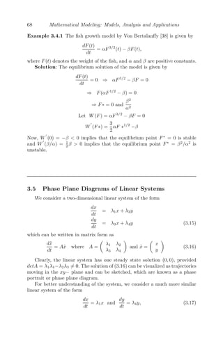
Example 3.4.1 The fish growth model by Von Bertalanffy [38] is given by
dF(t)
dt
= αF3/2
(t) − βF(t),
where F(t) denotes the weight of the fish, and α and β are positive constants.
Solution: The equilibrium solution of the model is given by
dF(t)
dt
= 0 ⇒ αF3/2
− βF = 0
⇒ F(αF1/2
− β) = 0
⇒ F∗ = 0 and
β2
α2
Let W(F) = αF3/2
− βF = 0
W
(F∗) =
3
2
αF ∗1/2
−β
Now, W
(0) = −β 0 implies that the equilibrium point F∗
= 0 is stable
and W
(β/α) = 1
2 β 0 implies that the equilibrium point F∗
= β2
/α2
is
unstable.
3.5 Phase Plane Diagrams of Linear Systems
We consider a two-dimensional linear system of the form
dx
dt
= λ1x + λ2y
dy
dt
= λ3x + λ4y (3.15)
which can be written in matrix form as
dx̃
dt
= Ax̃ where A =
λ1 λ2
λ3 λ4
and x̃ =
x
y
(3.16)
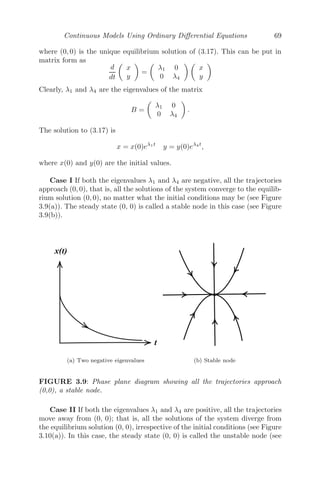
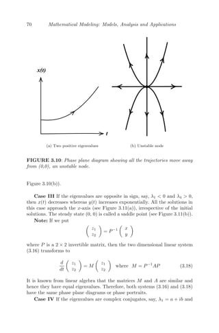
Clearly, the linear system has one steady state solution (0, 0), provided
detA = λ1λ4−λ2λ3 = 0. The solution of (3.16) can be visualized as trajectories
moving in the xy− plane and can be sketched, which are known as a phase
portrait or phase plane diagram.
For better understanding of the system, we consider a much more similar
linear system of the form
dx
dt
= λ1x and
dy
dt
= λ4y, (3.17)

116. Continuous Models Using Ordinary Differential Equations 69
where (0, 0) is the unique equilibrium solution of (3.17). This can be put in
matrix form as
d
dt
x
y
=
λ1 0
0 λ4
x
y
Clearly, λ1 and λ4 are the eigenvalues of the matrix
B =
λ1 0
0 λ4
.
The solution to (3.17) is
x = x(0)eλ1t
y = y(0)eλ4t
,
where x(0) and y(0) are the initial values.
Case I If both the eigenvalues λ1 and λ4 are negative, all the trajectories
approach (0, 0), that is, all the solutions of the system converge to the equilib-
rium solution (0, 0), no matter what the initial conditions may be (see Figure
3.9(a)). The steady state (0, 0) is called a stable node in this case (see Figure
3.9(b)).
(a) Two negative eigenvalues (b) Stable node
FIGURE 3.9: Phase plane diagram showing all the trajectories approach
(0,0), a stable node.
Case II If both the eigenvalues λ1 and λ4 are positive, all the trajectories
move away from (0, 0); that is, all the solutions of the system diverge from
the equilibrium solution (0, 0), irrespective of the initial conditions (see Figure
3.10(a)). In this case, the steady state (0, 0) is called the unstable node (see

117. 70 Mathematical Modeling: Models, Analysis and Applications
(a) Two positive eigenvalues (b) Unstable node
FIGURE 3.10: Phase plane diagram showing all the trajectories move away
from (0,0), an unstable node.
Figure 3.10(b)).
Case III If the eigenvalues are opposite in sign, say, λ1 0 and λ4 0,
then x(t) decreases whereas y(t) increases exponentially. All the solutions in
this case approach the x-axis (see Figure 3.11(a)), irrespective of the initial
solutions. The steady state (0, 0) is called a saddle point (see Figure 3.11(b)).
Note: If we put
z1
z2
= P−1
x
y
where P is a 2 × 2 invertible matrix, then the two dimensional linear system
(3.16) transforms to
d
dt
z1
z2
= M
z1
z2
where M = P−1
AP (3.18)
It is known from linear algebra that the matrices M and A are similar and
hence they have equal eigenvalues. Therefore, both systems (3.16) and (3.18)
have the same phase plane diagrams or phase portraits.
Case IV If the eigenvalues are complex conjugates, say, λ1 = a + ib and

118. Continuous Models Using Ordinary Differential Equations 71
(a) One positive and one negative
eigenvalue
(b) A saddle point
FIGURE 3.11: Phase plane diagram showing all the trajectories approach
the x-axis, a saddle point.
λ4 = a − ib, then the solutions are of the form
x(t) = x(0)eat
(cos b + i sin b)
y(t) = y(0)eat
(cos b − isin b)
(i) If a 0, then both the eigenvalues have negative real parts and the
term eat
decays for increasing t. In this case, all the trajectories spiral towards
the steady state (0, 0), irrespective of the initial conditions (see Figure 3.12(a))
and the steady state is known as a stable spiral or stable focus (see Figure
3.12(b)).
(ii) If a 0, both the eigenvalues have positive real parts and the term
eat
grows exponentially for t 0. In this case, all the trajectories spiral away
from the steady state (0, 0), irrespective of the initial conditions (see Figure
3.13(a)) and the steady state is called an unstable spiral or unstable focus (see
Figure 3.13(b)).
(iii) If a = 0, both the eigenvalues are purely imaginary. In this case, all
the trajectories are closed orbits about the steady state (0, 0). The solutions
are periodic (see Figure 3.14(a)) and the steady state is called a center (see
Figure 3.14(b)).

119. 72 Mathematical Modeling: Models, Analysis and Applications
(a) Eigenvalues with negative real
parts
(b) Stable focus
FIGURE 3.12: Phase plane diagram showing all the trajectories spiral to-
wards (0,0), a stable spiral or a stable focus.
3.6 Bifurcations
Consider a system of the form
dx
dt
= f(x, μ) where x ∈ Rn
and μ ∈ R.
The word bifurcation was introduced by Poincare, a French mathematician,
in the field of non-linear dynamics. He used this word to indicate qualitative
changes in the behavior of systems, where one or more system parameters are
varied. Mathematically, this means when the parameter μ crosses some point
μ = μ∗
, the phase portrait of the system for μ μ∗
is topologically different
from the phase portrait of the system for μ μ∗
. The point μ = μ∗
is called
a bifurcation point at which the system undergoes a bifurcation.
Different types of local bifurcations will be discussed now. By local bifur-
cations, it is meant that the qualitative changes occur in the neighborhood
of equilibria (fixed points) or periodic orbits as the system parameter passes
through the critical threshold μ = μ∗
. The local bifurcations of fixed points
(equilibrium points) are classified into static bifurcations or dynamic bifurca-
tions. Saddle-node bifurcation, pitchfork bifurcation and transcritical bifur-
cation are examples of static bifurcations as only branches of fixed points or
static solutions meet. Hopf bifurcation is an example of dynamic bifurcation.

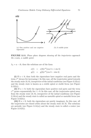
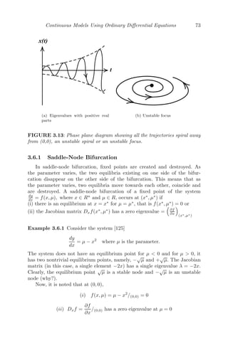
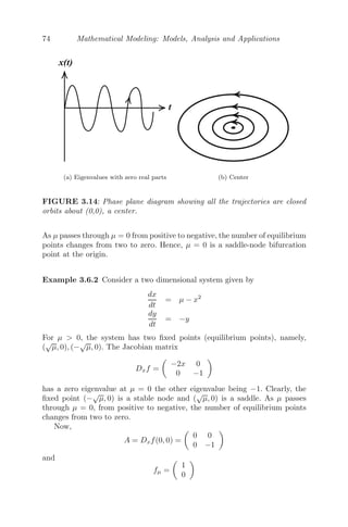
120. Continuous Models Using Ordinary Differential Equations 73
(a) Eigenvalues with positive real
parts
(b) Unstable focus
FIGURE 3.13: Phase plane diagram showing all the trajectories spiral away
from (0,0), an unstable spiral or an unstable focus.
3.6.1 Saddle-Node Bifurcation
In saddle-node bifurcation, fixed points are created and destroyed. As
the parameter varies, the two equilibria existing on one side of the bifur-
cation disappear on the other side of the bifurcation. This means that as
the parameter varies, two equilibria move towards each other, coincide and
are destroyed. A saddle-node bifurcation of a fixed point of the system
dy
dx = f(x, μ), where x ∈ Rn
and μ ∈ R, occurs at (x∗
, μ∗
) if
(i) there is an equilibrium at x = x∗
for μ = μ∗
, that is f(x∗
, μ∗
) = 0 or
(ii) the Jacobian matrix Dxf(x∗
, μ∗
) has a zero eigenvalue =
∂f
∂x
(x∗,μ∗)
Example 3.6.1 Consider the system [125]
dy
dx
= μ − x2
where μ is the parameter.
The system does not have an equilibrium point for μ 0 and for μ 0, it
has two nontrivial equilibrium points, namely, −
√
μ and +
√
μ. The Jacobian
matrix (in this case, a single element −2x) has a single eigenvalue λ = −2x.
Clearly, the equilibrium point
√
μ is a stable node and −
√
μ is an unstable
node (why?).
Now, it is noted that at (0, 0),
(i) f(x, μ) = μ − x2
/(0,0) = 0
(ii) Dxf =
∂f
∂x
/(0,0) has a zero eigenvalue at μ = 0

121. 74 Mathematical Modeling: Models, Analysis and Applications
(a) Eigenvalues with zero real parts (b) Center
FIGURE 3.14: Phase plane diagram showing all the trajectories are closed
orbits about (0,0), a center.
As μ passes through μ = 0 from positive to negative, the number of equilibrium
points changes from two to zero. Hence, μ = 0 is a saddle-node bifurcation
point at the origin.
Example 3.6.2 Consider a two dimensional system given by
dx
dt
= μ − x2
dy
dt
= −y
For μ 0, the system has two fixed points (equilibrium points), namely,
(
√
μ, 0), (−
√
μ, 0). The Jacobian matrix
Dxf =
−2x 0
0 −1
has a zero eigenvalue at μ = 0 the other eigenvalue being −1. Clearly, the
fixed point (−
√
μ, 0) is a stable node and (
√
μ, 0) is a saddle. As μ passes
through μ = 0, from positive to negative, the number of equilibrium points
changes from two to zero.
Now,
A = Dxf(0, 0) =
0 0
0 −1
and
fμ =
1
0

122. Continuous Models Using Ordinary Differential Equations 75
Following Sotomayor’s theorem [98, 125], let ν = w = (1, 0)T
, then
wT
fμ(0, 0) =
1 0
1
0
= 1 = 0
and
wT
[D2
f(0, 0)(ν, w)] =
1 0
−2 0
0 0
1
0
= −2 = 0
Therefore, the system experiences a saddle-node bifurcation at the equi-
librium point (0, 0) as the parameter μ passes through μ = 0 (see Figure
3.15).
1.0 0.5 0.5 1.0
Μ
1.0
0.5
0.5
1.0
x
SaddleNode Bifurcation
FIGURE 3.15: A saddle-node bifurcation as μ passes through μ = 0 from
positive to negative.
3.6.2 Transcritical Bifurcation
In transcritical bifurcation, the fixed points change their stability as the
bifurcation parameter is varied. The fixed points of the system exist for all
parameter values and can never be destroyed.
Example 3.6.3 Consider a system given by [125]
dx
dt
= μx − x2
dy
dt
= −y

123. 76 Mathematical Modeling: Models, Analysis and Applications
The system has two fixed points, namely, (0, 0) and (μ, 0). The Jacobian
matrix
Dxf =
μ − 2x 0
0 −1
Now,
A = Dxf(0, 0) =
μ 0
0 −1
and fμ =
x
0
Clearly, A has a simple eigenvalue at μ = 0 and let υ =
1 0
T
and
w =
1 0
T
be the eigenvectors of A and AT
respectively, corresponding
to the eigenvalue λ = 0. Following Sotomayor’s theorem [98, 125], we have
wT
fμ(0, 0) =
1 0
0
0
= 0
wT
[Dfμ(0, 0)υ] =
1 0
1
0
wT
[D2
f(0, 0)(υ, υ)] =
1 0
−2 0
0 0
1
0
= −2 = 0
Therefore, the system experiences a transcritical bifurcation at the equilibrium
point (0 ,0) as the parameter μ passes through μ = 0.
1.0 0.5 0.0 0.5 1.0
1.0
0.5
0.0
0.5
1.0
Μ
x
Transcritical Bifurcation
FIGURE 3.16: A transcritical bifurcation at the equilibrium point (0,0) as
the parameter μ passes through μ = 0.
For μ 0, the equilibrium point (μ, 0) is unstable and (0, 0) is stable

124. Continuous Models Using Ordinary Differential Equations 77
with increasing μ. The unstable fixed point (μ, 0) approaches the origin and
coalesces with it when μ = 0. And, when μ 0, the fixed point (μ, 0) becomes
stable and the origin becomes unstable. Thus, in a transcritical bifurcation,
there is a stability switch between two points of equilibria (see Figure 3.16).
3.6.3 Pitchfork Bifurcation
A pitchfork bifurcation is a particular type of local bifurcation (possible in
dynamical systems) that have a symmetry. In such cases equilibrium points
appear and disappear in symmetrical pairs. There are two types of pitchfork
bifurcations, namely supercritical and subcritical.
Example 3.6.4 Consider the system [125]
dx
dt
= f(x; μ) = μx − x3
dy
dt
= −y
There are three fixed points, namely, (0, 0), (+
√
μ, 0) and (−
√
μ, 0).
The Jacobian matrix
Dxf =
μ − 3x2
0
0 −1
has the eigenvalue λ = μ at (0, 0) and λ = −2μ at (±
√
μ, 0).
Now,
A = Dxf(0, 0) =
μ 0
0 −1
and fμ =
x
0
Clearly, A has a simple eigenvalue at μ = 0 and let υ =
1 0
T
and
w =
1 0
T
be the eigenvectors of A and AT
respectively, corresponding
to the eigenvalue λ = 0 (since μ = 0). Following Sotomayor’s theorem [125, 98],
we get,
wT
fμ(0, 0) =
1 0
0
0
= 0
wT
[Dfμ(0, 0)υ] =
1 0
1
0
wT
[D2
f(0, 0)(υ, υ)] =
1 0
0 0
0 0
1
0
= 0
wT
[D3
f(0, 0)(υ, υ, υ)] =
1 0
−6 0
0 0
1
0
= −6 = 0

125. 78 Mathematical Modeling: Models, Analysis and Applications
Therefore, the system experiences a pitchfork bifurcation at the equilibrium
point (0, 0) as the parameter μ varies through the bifurcation point μ = 0.
For μ 0, the trivial fixed point (0, 0) is stable and unstable for μ 0.
Therefore, there is a change of stability of the trivial fixed point as μ passes
through μ = 0.
For μ 0, the origin is the only equilibrium point. But for μ 0, two new
stable equilibrium points appear on either side of the origin, points symmetri-
cally located at (+
√
μ, 0) and (+
√
μ, 0). This is an example of a supercritical
pitchfork bifurcation (see Figure 3.17(a)).
The term “pitchfork” is due to the fact that the bifurcating non-trivial
branches have the geometry of a pitchfork at (0, 0). The characteristic of a
supercritical pitchfork bifurcation is that there is a branch of stable equilib-
rium points (locally) on one side of the bifurcation point (μ = 0, in this case)
and two branches of stable equilibrium points and a branch of unstable equi-
librium points on the other side of the bifurcation point.
1.0 0.5 0.0 0.5 1.0
1.0
0.5
0.0
0.5
1.0
Μ
x
Supercritical Pitchfork
(a) Supercritical pitchfork bifurcation
1.0 0.5 0.0 0.5 1.0
1.0
0.5
0.0
0.5
1.0
Μ
x
Subcritical Pitchfork
(b) Subcritical pitchfork bifurcation
FIGURE 3.17: Pitchfork bifurcation at the equilibrium point (0,0) as the
parameter μ passes through μ = 0.
Note: Readers may look into the system ẋ = μx+x3
, ẏ = −y for subcriti-
cal pitchfork bifurcation. The characteristic of subcritical pitchfork bifurcation
is that there are two branches of unstable equilibrium points and a branch of
stable equilibrium points on one side of the bifurcation point and a branch
of unstable equilibrium points on the other side of the bifurcation point (see
Figure 3.17(b)).

126. Continuous Models Using Ordinary Differential Equations 79
3.6.4 Hopf Bifurcation
We consider a two dimensional system of the form
dx
dt
= f(x, y, μ)
dy
dt
= g(x, y, μ)
where μ is a parameter. The system has a fixed point (x∗
, y∗
), which may
depend on μ. Let the eigenvalues of the linearized system about this fixed
point be given by
λ(μ) = α(μ) + iβ(μ) and λ̄(μ) = α(μ) − iβ(μ)
A Hopf bifurcation is a local bifurcation, which occurs when a conjugated
complex pair of eigenvalues of the linearization around the equilibrium point
crosses the boundary of stability, that is, the imaginary axis of the complex
plane. Mathematically, it means that a Hopf bifurcation of the fixed point of
the two dimensional system occurs at some critical value of the parameter,
μ = μc (say), if the following conditions are satisfied:
(i) f(x∗
, y∗
, μc) = 0, g(x∗
, y∗
, μc) = 0
(ii) The Jacobian matrix
∂f
∂x
∂f
∂y
∂g
∂x
∂g
∂y
(x∗,y∗)
has a pair of purely imaginary eigenvalues ±iω at (x∗
, y∗
, μc), that is, (α(μc) =
0, β(μc) = 0)
(iii) dα(μ)
dμ = 0 at μ = μc
Example 3.6.5 Consider the system
dx
dt
= μx − y +
x +
3
2
y
x2
+ y2
dy
dt
= x + μy +
3
2
x − y
x2
+ y2
Clearly, the origin (0,0) is the equilibrium point. The linearization about the
origin gives
dx
dt
= μx − y
dy
dt
= x + μy
whose Jacobian matrix is
μ −1
1 μ
. The eigenvalues are μ ± i. Thus, we

127. 80 Mathematical Modeling: Models, Analysis and Applications
1.0 0.5 0.0 0.5 1.0
1.0
0.5
0.0
0.5
1.0
Μ
x
Supercritical Hopf
(a) Supercritical Hopf bifurcation
2 1 0 1 2
1.5
1.0
0.5
0.0
0.5
1.0
1.5
Μ
x
Subcritical Hopf
(b) Subcritical Hopf bifurcation
FIGURE 3.18: The system exhibits Hopf bifurcation as the parameter μ
passes through μ = 0.
get a stable focus if μ 0 and an unstable one if μ 0. Also, d(μ)
dμ = 1(= 0)
at μ = 0. As μ passes through μ = 0, the dynamics of the system change from
stable focus to an unstable one, and the eigenvalues change from negative to
positive as μ passes through μ = 0, which is the bifurcation point. It is to be
noted that all the three conditions for Hopf bifurcation are satisfied. Hence,
we conclude that the system undergoes Hopf bifurcation at the point μ = 0
(see Figure 3.18).
3.7 Miscellaneous Examples
Problem 3.7.1 The generalized Verhulst population model, with crowding ef-
fect of the form (−βNα
) is given by
dN
dt
= rN − βNα
(α 1)
Obtain the steady state solution and check for stability. Also, solve the model
for N and predict the behavior of the population for a long period of time.
Solution: The steady state solution is given by
dN
dt
= 0
⇒ N(r − βN(α−1)
) = 0
⇒ N∗
= 0 and N∗
=
r
β
1
α−1
.

128. Continuous Models Using Ordinary Differential Equations 81
Let f(N) = rN − βNα
, then, f
(N) = r − βαNα−1
.
Now, f
(0) = r 0 ⇒ the system is unstable about N∗
= 0 and
f
r
β
1
α−1
= r(1 − α) 0 ⇒ the system is unstable about N∗
=
r
β
1
α−1
.
Putting N(α−1)
= k in
dN
dt
= rN − βNα
, we get,
dk
k(α − 1)(r − kβ)
= dt
⇒
(r − kβ + kβ)
k(α − 1)(r − kβ)
dk = dt
⇒ (
1
k
+
β
r − kβ
)dk = r(α − 1)dt
Integrating, ln(k) − ln(r − kβ) = rt(α − 1) + c
⇒ ln
k
r − kβ
= rt(α − 1) + c
⇒
k
r − kβ
= c1
ert(α−1)
⇒ Nα−1
=
rc1
ert(α−1)
1 + βc1ert(α−1)
For large time, that is, as, t → ∞, N(α−1)
→
r
β
⇒ N →
r
β
1
α−1
Problem 3.7.2 A spherical raindrop of radius a falls from a height h and
accumulates moisture from the atmosphere as it descends, thereby increasing
the radius of the spherical raindrop at a rate λa. Show that the radius of
the raindrop is λa
2h
g (1 +
1 + g
2hλ2 ), when it hits the ground, g being the
acceleration due to gravity.
Solution: Let M be the mass of the raindrop, then M = 4
3 πa3
ρ, a is the
radius and ρ is the density.
Now, dr
dt = λa ⇒ r = a(1 + λt), r(0) = a.
Therefore, mass at time t = 4
3 πr3
ρ = M(1 + λt)3
.
Equation of Motion:
d
dt
M(1 + λt)3
ẋ
= M(1 + λt)3
g

129. 82 Mathematical Modeling: Models, Analysis and Applications
Integrating we get,
ẋ(t) =
g
4λ
1 + λt −
1
(1 + λt)3
, ẋ(0) = 0.
Integrating again, x(t) =
g
8λ2
1 + λt −
1
1 + λt
− 2
, x(0) = 0.
⇒ x(t) =
g
8λ2
1 + λt −
1
1 + λt
2
=
g
8λ2
r
a
−
a
r
2
When the raindrop reaches the ground, x = h. This implies
r2
− 2λa
2h
g
r − a2
= 0
⇒ r = λa
2h
g
(1 +
1 +
g
2hλ2
)
Problem 3.7.3 An elastic string of unstretched length a and modulus of elas-
ticity λ is fixed to a point on a smooth horizontal table and the other end is
tied to a particle of mass m, which is lying on the table. The particle is pulled
to a distance, where the extension of the string is b and then let go. Find the
time of complete oscillation.
FIGURE 3.19: The motion of an elastic string lying on a smooth horizontal
table.
Solution: We consider an elastic string, whose unstretched length is
OA1 = a (see Figure 3.19) and modulus of elasticity is λ. One end of the
elastic string is fixed to a point on a smooth horizontal table and the other
end is attached to a particle of mass m, which is lying on the table. The par-
ticle is now pulled to a distance where the extension of the string is b(A1B1)
and then let go. Let P be the position of the particle at any time t, such that
OP = x.
Then, the equation of motion satisfies the differential equation
m
d2
x
dt2
= −T

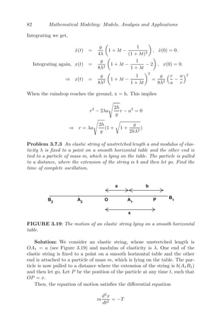
130. Continuous Models Using Ordinary Differential Equations 83
where T = tension in the string (a x a + b)
= (modulus of elasticity) ×
increase of length
original length
= λ
x − a
a
[by Hooke’s law].
∴
d2
(x − a)
dt2
= −
λ
am
(x − a), (3.19)
which shows that the motion is simple harmonic about the center A1, ampli-
tude b. The solution of (3.19) is
x − a = K1cos
λ
am
t + K2 sin
λ
am
t
where K1 and K2 are arbitrary constants.
dx
dt
= −K1
λ
am
sin
λ
am
t + K2
λ
am
cos
λ
am
t
When t = 0, the particle was at B1, where x = a + b and dx
dt = 0
⇒ b = K1 and 0 = K2
∴ x − a = b cos
λ
am
t
(3.20)
and
dx
dt
= −b
λ
am
sin
λ
am
t
(3.21)
Let T1 be the time taken by the particle from the point B1 to A1. Then from
(3.20) we get,
0 = b cos
λ
am
T1
[putting x = a]
⇒
λ
am
T1 =
π
2
⇒ T1 =
λ
am
π
2
.
The velocity of the particle at the point A1 is given by (3.21) as
dx
dt
= −b
λ
am
sin
λ
am
T1
= −b
λ
am
sin
π
2
= −b
λ
am
.

131. 84 Mathematical Modeling: Models, Analysis and Applications
Therefore, the particle reaches its maximum velocity at point A1. At this
point the elastic string becomes slack and the tension ceases. The equation
of motion given by equation (3.19) does not hold any more and the particle
moves with uniform speed b
λ
am from the point A1, until it reaches the point
A2. Once it crosses the point A2, the string again becomes taut and tension
now acts in the direction A2O. The velocity slowly decreases and goes to zero
at the point B2 such that OB2 = OB1. The particle then retraces its path
and reaches B1 and this cycle of motion goes on.
Now, time taken from A1 to O = Distance
Speed = a
b
√ λ
am
There, time taken from B1 to O
=
am
λ
π
2
+
a
b
λ
am
=
π
2
+
a
b
am
λ
Hence, time for complete oscillation is 4 times the time from B1 to O
= 4
π
2
+
a
b
am
λ
.
Problem 3.7.4 A seasonal growth model is given by
dS
dt
= αS cos(βt)
where α and β are constants. Comment on the behavior of the solution S(t)
of this model.
Solution: Given that
dS
dt
= αS cos(βt)
⇒
dS
S
= α cos(βt)dt
⇒ ln S =
α
β
sin(βt) + C
⇒ S(t) = c1e
α
β sin(βt) where c1 = eC
.
Thus, S(t) will be an exponential function, the power of which varies as a
sinusoidal function with increasing amplitude.
Problem 3.7.5 Let G be the amount of glucose in the bloodstream at any
time t, α( 0) is the constant rate of infusion and β( 0) is the removal
rate of glucose from the bloodstream. Using differential equations, construct a

132. Continuous Models Using Ordinary Differential Equations 85
mathematical model of the infusion of glucose into the bloodstream. By solving
the differential equation, predict the glucose level in the bloodstream and show
that G → α
β as t → ∞.
Solution: The required model is
dG
dt
= α − βG
⇒
dG
α − βG
= dt
⇒
ln(α − βG)
−β
= t + c1
⇒ G(t) =
α
β
−
c1e−βt
β
At t → ∞ , G → α
β , since e−βt
→ 0.
Problem 3.7.6 Suppose in a chemical reaction two substances, M1 and M2,
react in equal amounts to form a compound M3. Let C(t) be the concentration
of the compound M3 at time t, which satisfies the differential equation
dC
dt
= r(a − C)(b − C)
where r is a positive constant; a and b are initial concentrations of M1 and
M2 at time t = 0. Obtain the concentration of M3 as a function of time for
t 0, assuming C(0) = 0. Also determine the limiting concentration when
a = 9 and b = 14.
Solution: Given that,
dC
dt
= r(a − C)(b − C)
⇒
dC
(a − C)(b − C)
= rdt
Integrating, we get, C = (a + b) − (a − b)
ae(a−b)rt
+ b
ae(a−b)rt − b
For the particular choice of a = 9, b = 14 and for the limiting concentration
we have,
C∞ = (a + b) − (a − b)(
0 + b
0 − b
) = 2a = 18, as t → ∞.
Problem 3.7.7 Suppose a single infected individual migrates into a commu-
nity containing n individuals susceptible to a disease. The infected individual

133. 86 Mathematical Modeling: Models, Analysis and Applications
spreads the disease to all susceptible. If S(t) be the number of susceptible at
time t, then
dS
dt
= −rS(n + 1 − S) with S(0) = n.
and r is a positive constant which measures the infection. Obtain the solution
of this model and comment.
Solution: Given that, dS
dt = −rS(n + 1 − S)
dS
dt
= −rS(n + 1 − S)
⇒
1
n + 1
1
S
+
1
n + S − 1
dS = −
rdt
⇒ ln
S
n(n + 1 − S)
= −(n + 1)rt, S(0) = n.
S(t) =
n(n + 1)
e(n+1)rt + n
As t → ∞, S → 0, since r is a positive constant. Hence, we conclude that after
a long time, all susceptible people will convert into the infected people.
Problem 3.7.8 The price of sugar, initially 50 per kg, is p(t) per kg. After t
weeks, the demand is D = 120 − 2p + 5dp
dt and the supply S = 3p − 30 + 50dp
dt
thousand per week. Show that, for D = S, the price of sugar must vary over
time accordingly to the law p = 30 + 20e− t
9 . Predict the prices of the sugar
after 15 weeks and 60 weeks. Draw a graph to show the approach of the price
to the equilibrium value.
Solution: For D = S, we get,
120 − 2p + 5
dp
dt
= 3p − 30 + 50
dp
dt
9
dp
dt
+ p = 30
⇒ p(t) = Ae− t
9 + 30
p(t) = 20e− t
9 + 30, P(0) = 50.
Clearly, p(15) = 33.78 and p(60) = 30.03. Both analytically and graphi-
cally, we see that as t → ∞, p(t) → 30 (see Figure 3.20).
Problem 3.7.9 We consider two trees that are growing independently, sup-
ported by independent fixed supplies of substrate. Let p1(t) and p2(t) be the dry

134. Continuous Models Using Ordinary Differential Equations 87
20 40 60 80 100
25
30
35
40
45
50
FIGURE 3.20: The price of the sugar approaching a steady value of 30 as
time increases.
weights of the trees at time t respectively. The system of differential equations
governing the scenario is given by
dp1
dt
= α1p1(k1 − p1)
dp2
dt
= α2p2(k2 − p2)
(i) Explain the parameters α1, α2, k1 and k2.
(ii) Obtain the solution for p1(t).
(iii) Taking α1 = α2 = 0.1, k1 = 7, k2 = 10 and with different initial conditions
(p1(0), p2(0)), plot the solution curves in the p1p2 plane in the rectangle 0
p1 10, 0 p2 10.
Solution (i) Here, α1 is the rate at which the dry weight p1 of Tree I
decreases on its own, k1 being its carrying capacity and α1k1 is the rate of
increase of the weight of Tree I or the natural growth rate. Similarly, α2 is the
rate at which the dry weight p2 of Tree II decreases on its own i.e. the growth
is restricted and k2 is the carrying capacity. α2k2 is the rate of increase of
weight of Tree II or the natural growth rate.

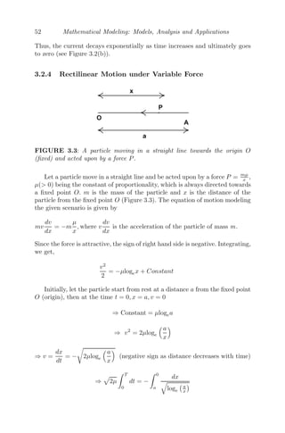
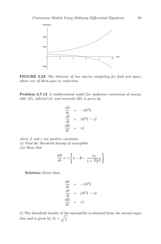
135. 88 Mathematical Modeling: Models, Analysis and Applications
0 2 4 6 8 10
0
2
4
6
8
10
FIGURE 3.21: The dynamics of the independent trees for different initial
conditions.
(ii) Given that
dp1
dt
= α1p1(k1 − p1)
dp2
dt
= α2p2(k2 − p2)
Now,
dp1
dt
= α1p1(k1 − p1)
⇒
dp1
p1(k1 − p1)
= α1dt
⇒ ln(
p1
k1 − p1
) = k1α1t + c1
⇒ p1 =
k1
1 + Ce−k1α1t
, where C = ec1
.
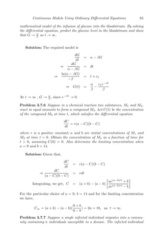
Figure 3.21 shows the growth of the independent trees in the p1p2 plane
in the rectangle 0 p1 10, 0 p2 10 for given initial values.
Problem 3.7.10 Consider the pricing policy of edible oil, where the manu-
facturers stock the product to meet any sudden unexpected demand from cus-
tomers. Let S(t) and Q(t) be the sales forecast and production forecast respec-
tively and p(t) be the price of edible oil at any time t. Then the general pricing
policy is given by
S(t) = α1 − β1p − γ1
dp
dt
Q(t) = α2 − β2p − γ2
dp
dt
dp
dt
= −γ[L(t) − L0]

136. Continuous Models Using Ordinary Differential Equations 89
Here, α1, α2, β1, β2, γ1, γ2, δ are positive constants, L is the inventory level and
L0 the desired optimum inventory level. The changes in inventory follow the
law
dL
dt
= Q − S.
Show that the equation
d2
p
dt2
+ δ(γ1 − γ2)
dp
dt
+ δ(β1 − β2)p = δ(α1 − α2)
gives the forecast price. Hence, deduce that if γ1 γ2, β1 β2, the price
tends to be stable as t increases.
Solution: Given that,
dL
dt
= Q − S
S(t) = α1 − β1p − γ1
dp
dt
Q(t) = α2 − β2p − γ2
dp
dt
⇒
dL
dt
= (α2 − α1) − p(β2 − β1) − (γ2 − γ1)
dp
dt
Also,
dp
dt
= −γ[L(t) − L0]
⇒
d2
p
dt2
= −δ
dL(t)
dt
⇒
d2
p
dt2
= −δ
(α2 − α1) − p(β2 − β1) − (γ2 − γ1)
dp
dt
⇒
d2
p
dt2
+ δ(γ1 − γ2)
dp
dt
+ δ(β1 − β2)p = δ(α1 − α2), (3.22)
which gives the forecast price. Equation (3.22) is a second order ordinary
differential equation with constant coefficients, whose complementary function
is
Ae−m1t
+ Be−m2t
where m1, m2 = −δ(γ1 − γ2) ± δ
(γ1 − γ2)2 − 4
(β1 − β2)
δ
,
and both are negative as γ1 γ2 and β1 β2. The particular integral is
δ(α1−α2)
δ(β1−β2) . Therefore, the general solution of (3.22) is
p(t) = Ae−m1t
+ Be−m2t
+
δ(α1 − α2)
δ(β1 − β2)

137. 90 Mathematical Modeling: Models, Analysis and Applications
As t → ∞, p(t) tends to a steady value (α1−α2)
(β1−β2) , as both m1 and m2 are
negative.
Problem 3.7.11 Consider a model of species competing for food and space.
The governing equation is given by
dx
dt
= αx − βy
dy
dt
= γy − δx
where x and y are two competing species, α, β, γ, δ are positive constants.
(i) show that
d2
x
dt2
− (α + γ)
dx
dt
+ (αγ − βδ)x = 0
and solve for x.
(ii) Also, find the solution for y.
(iii) If at t = 0, x = 100 and y = 200, obtain graphically the time when one
species is eliminated (take α = 0.2, β = 0.1, γ = 0.2, δ = 0.1).
Solution:(i) Given that,
dx
dt
= αx − βy and
dy
dt
= γy − δx
⇒
d2
x
dt2
= α
dx
dt
− β
dy
dt
= α
dx
dt
− β(γy − δx)
= α
dx
dt
− γ(−
dx
dt
− αx) + δβx
= α
dx
dt
+ γ
dx
dt
− αβx + δβx
⇒
d2
x
dt2
− (α + γ)
dx
dt
+ (αγ − βδ)x = 0
This is a second order ordinary differential equation with constant coefficients,
whose auxiliary equation is
m2
− (α + γ)m + (αγ − βδ) = 0.
Solving, we get, m1, m2 =
(α + γ) ±
γ2 + α2 + 4βδ − 2αγ
2
Therefore, the required solution is
x(t) = Aem1t
+ Bem2t
(ii) y(t) = Cem3t
+ Dem4t
(Do yourself).
(iii) The model is solved numerically with α = 0.2, β = 0.1, γ = 0.2, δ = 0.1
and Figure 3.22 shows that species x goes to extinction after 5.5 units of time.

138. Continuous Models Using Ordinary Differential Equations 91
2 4 6 8 10
Time
1000
1000
2000
Population
FIGURE 3.22: The behavior of two species competing for food and space,
where one of them goes to extinction.
Problem 3.7.12 A mathematical model for epidemics consisting of suscep-
tible (S), infected (I) and removals (R) is given by
dS
dt
= −βS2
I
dI
dt
= βS2
I − γI
dR
dt
= γI
where β and γ are positive constants.
(i) Find the threshold density of susceptible.
(ii) Show that
dR
dt
= γ
n − R −
x0
1 + Rx0β
γ
Solution: Given that,
dS
dt
= −βS2
I
dI
dt
= βS2
I − γI
dR
dt
= γI
(i) The threshold density of the susceptible is obtained from the second equa-
tion and is given by S† =
γ
β

139. 92 Mathematical Modeling: Models, Analysis and Applications
(ii) Adding the three equations we get,
dS
dt
+
dI
dt
+
dR
dt
= 0
⇒ S+I+R =n (constant).
Now,
dS
dt
= −βS2
I = −βS2 1
γ
dR
dt
⇒
dS
S2
= −
β
γ
dR
Integrating we get,
1
S
=
β
γ
R +
1
S0
, since S(0) = S0 and R(0) = 0.
⇒ S(t) =
S0
1 + βS0R
γ
Now,
dR
dt
= γI = γ(n − R − S) = γ(n − R −
βS0R
γ
)
Problem 3.7.13 The British Museum was authorized in 1988 by the Vatican
to date a cloth relic known as the Shroud of Turin (possibly, the burial shroud
of Jesus of Nazareth), which contains the negative image of a human body,
widely believed to be that of Jesus. The British Museum’s report confirmed that
the cloth fibres contained between 92% and 93% of their original C14
. Estimate
the approximate age of the Shroud, using the method of carbon dating. Assume
that the half-life of radioactive C14
is 5730 years.
Solution: Let A(t) be the amount of C14
present in the sample at any
time t, then
dA
dt
= −λA (following radioactive decay law)
⇒ A(t) = A0e−λt
,
where λ is the decay constant of the sample and is given by
λ =
1
τ
loge 2, τ being the half-life of C14
=
loge 2
5730
≈ 0.000121 (see Section 3.2.1).
Therefore, the fraction of the original C14
present after t-years is
A(t) = A0e−0.000121t
⇒ t = −
1
0.000121
loge
A(t)
A0
,

140. Continuous Models Using Ordinary Differential Equations 93
A0 = A(0) being the units of C14
present at time t = 0. Taking A(t)
A0
= 0.92
and 0.93, we get,
t1 = −
1
0.000121
loge (0.92) ≈ 689 and
t2 = −
1
0.000121
loge (0.93) ≈ 600.
Therefore, from the test conducted by the British Museum in 1988, it was
concluded that the Shroud was between 600 and 689 years old, thereby plac-
ing its origin between 1299 A.D. and 1388 A.D. Hence, by the method of C14
dating, the Shroud of Turin cannot be the burial shroud of Jesus of Nazareth.
Problem 3.7.14 We consider a competition model of the form
dx
dt
= 0.05x
1 −
x
250000
− axy
dy
dt
= 0.08y
1 −
y
400000
− axy
where x denotes the population of blue whales and y denotes the population of
fin whales.
(i) Find the equilibrium points for a = 10−8
.
(ii) Solve the model numerically, assuming x(0) = 6000 and y(0) = 60, 000
for a = 10−8
and 10−6
and conclude on the dynamics of the system.
(iii) Assuming that x(0) = 6000, and y(0) = 60000 and a = 10−7
, simulate to
find out what happens to the two species of whales over the long term.
(iv) Currently, the intrinsic growth rate of the blue whale is 5% per year.
Assuming a = 10−8
and intrinsic growth rates to be 2%, 3%, 4%, 6% and 7%
per year, solve the model numerically to comment on the dynamics of the two
species of whales.
(v) The effects of harvesting is now considered on the two whale populations.
Assuming a = 10−8
and E = 3000 boat days per year, resulting in the annual
harvest of qEx blue whales and qEy fin whales (q = catch ability coefficient =
10−5
), rewrite the model and find what happens to the two whale species over
the long term, by numerical simulation. Repeat the same process for E = 6000
boat days per year. Find the range of E for which the number of whales of
both species approach a non-zero equilibrium.
(vi) Taking E = 500, 1000, 1500, 2000, 2500, 3000, 4000, 4500, 5500, 6000, 7000
boat days, comment on which case results in the highest sustainable yield.
(vii) Assuming x(0) = 140000 and y(0) = 350000 (before mankind began to
harvest), find the minimum level of effort required to reduce the blue whales
to the level of around 6000 whales.

141. 94 Mathematical Modeling: Models, Analysis and Applications
(viii) Suppose the model is modified to
dx
dt
= 0.05x
x − Cx
x + Cx
1 −
x
k
− axy
dy
dt
= 0.08y
y − Cy
y + Cy
1 −
y
k
− axy
where Cx and Cy are the minimum viable population levels below which the
growth rates of the blue whale and fin whale are negative. Use numerical simu-
lation to comment on the coexistence of the two species of whales by assuming
a = 10−8
, Cx = 35000 and Cy = 16000. Find the equilibrium points and clas-
sify each of them as stable or unstable. What does the model predict about the
future of the two whale populations, assuming x(0) = 6000 and y(0) = 60000?
Suppose Cx = 1500 instead of 35000, what does the model predict now?
(ix) Krill, a tiny shrimp-like creature, is the principal food for blue whales,
which are of course devoured in massive amounts. Assuming that the krill
population grows at a rate of 30% per year in the absence of a predator (blue
whale) and decreases at a rate of 15% per year due to the presence of 200000
blue whales and the blue whale population grows at a rate of 3% per year,
formulate a mathematical model using differential equations. The maximum
sustainable population of krill is 600 tons/acre. Predict the dynamics of both
populations over time, if initially there are 6000 blue whales and 800 tons/acre
of krill.
Solution: (i) Equilibrium solutions are (0, 0); (250000, 0); (0, 400000) and
(230576, 388471).
(ii) The competition model of blue whales and fin whales is solved numeri-
cally. For a = 10−8
, both whales coexist (see Figure 3.23(a)) and for a = 10−6
,
the blue whale population dies out (see Figure 3.23(b)). For both cases, the
initial conditions are (x0, y0) = (6000, 60000).
(iii) This one is similar to (ii) and hence is left to the reader.
(iv) Figure 3.24 shows that with increasing growth rate r =
0.02, 0.03, 0.04, 0.06 and 0.07, the blue whales reach the steady state value
of 250000 at a faster rate.
(v) With harvesting taken into account, the modified model is given by
dx
dt
= 0.05x
1 −
x
250000
− axy − qEx
dy
dt
= 0.08y
1 −
y
400000
− axy − qEy
Figure 3.25 shows that when the number of boat days per year is increased

142. Continuous Models Using Ordinary Differential Equations 95
Species 2
Species 1
100 200 300 400 500
100000
200000
300000
400000
(a) Species behavior for a = 10−8
Species 2
Species 1
10 20 30 40 50
50000
100000
150000
200000
250000
300000
350000
(b) Species behavior for a = 10−6
FIGURE 3.23: The dynamics of blue whales and fin whales population com-
peting for food.
2%
3%
4%
6%
7%
Fin Whales
Blue Whales
100 200 300 400 500
100000
200000
300000
400000
FIGURE 3.24: The behavior of blue whales with increasing intrinsic growth
rate.
from 3000 to 6000, the fin whales survive but all the blue whales die out.
The non-zero equilibrium point (with E) is given by (230576 −
47.619E, 388471 − 47.619E) and both need to be positive, which implies
E min(4842.1, 8157.9) ≈ min(4842, 8158). Therefore, the range of E for
which the number of whales of both species approaches a non-zero equilib-
rium is 0 E 4842.
(vi) Left to the reader (mathematica code is given).
(vii) It can be easily checked that for a = 1.231 × 10−7
, the blue whales
reduce to the level of around 6000 whales.
(viii) With initial populations x(0) = 6000, y(0) = 60000 and a = 10−8
,
Cx = 35000, Cy = 16000, the model predicts that the fin whales survive and

143. 96 Mathematical Modeling: Models, Analysis and Applications
Fin Whales (E = 3000)
Blue Whales (E = 3000)
Fin Whales (E = 6000)
Blue Whales (E = 6000)
100 200 300 400 500
50000
100000
150000
200000
250000
FIGURE 3.25: The behavior of blue whales with increasing boat days, that
is, with increasing harvesting.
reach a steady state value while the blue whales die off (see Figure 3.26). Lin-
ear stability analysis about the points of equilibria is left to the reader.
20 40 60 80 100
1000
2000
3000
4000
5000
6000
20 40 60 80 100
100000
200000
300000
400000
FIGURE 3.26: The dynamics of the whales with minimum viable population
level with Cx = 35000 and Cy = 16000.
But with Cx = 1500 and Cy = 16000, both whales survive and reach
non-zero equilibria (see Figure 3.27).
(ix) Let K(t) be the krill population and x(t) be the population of blue
whales. Then, according to the problem, the model is given by
dK
dt
= 0.3K
1 −
K
600
− 0.15Kx
dx
dt
= 0.03x
1 −
x
200000
The krill goes to extinction while the blue whales reach a non-zero steady
state (see Figure 3.28).

144. Continuous Models Using Ordinary Differential Equations 97
Fin Whales
Blue Whales
50 100 150 200 250 300
100000
200000
300000
400000
FIGURE 3.27: The dynamics of the whales with minimum viable population
level with Cx = 1500 and Cy = 16000.
0.002 0.004 0.006 0.008 0.010
200
400
600
800
50 100 150 200 250 300
5000
10000
15000
20000
FIGURE 3.28: The dynamics between the predator blue whale and its prey
krill.
Problem 3.7.15 We consider a battle between two forces A and B. The mil-
itary strategy of wearing down the enemy by continued losses in personnel
(attrition) is due to infantry (direct fire) and artillery (area fire). We assume
that the loss in personnel due to direct fire is proportional to the number of
enemy infantry. We also assume that the attrition rate due to artillery is pro-
portional to the product of the two forces A and B. Also, force B has greater
weapon effectiveness than force A. The mathematical model of the above sce-
nario is given by
dx
dt
= −λay − λbxy
dy
dt
= −ax − bxy
where x and y are the number of personnel in force A and force B respec-
tively; a, b, λ( 1) are positive constants. Since weapon effectiveness of force

145. 98 Mathematical Modeling: Models, Analysis and Applications
B is more than force A, they cause more harm. Therefore, the rates in the
first equation are multiplied by some constant λ( 1). Solve the model numer-
ically by taking a = 0.05 and b = 0.005 for λ = 1.5, 2, 3 and 5, starting with
x(0) = 50 and y(0) = 30 and comment on the result.
Solution: (i) The model is solved numerically for different λ. For λ = 1.5,
the number of personnel y(t) of force B die within 10 units of time despite
having the greater weapon effectiveness than force A (see Figure 3.29(a)),
whereas for λ = 2.0, the number of personnel x(t) of force B die in 30 units of
time (see Figure 3.29(b)). For λ = 3.0 and 5.0, we observe similar dynamics,
only, personnel x(t) of force B die at a much faster rate with respect to units
of time (see Figure 3.29(c) and 3.29(d)).
A
10 20 30 40 50
50
100
150
200
B
x(t)
y(t)
20 40 60 80 100
20
40
60
80
C
Time
5 10 15 20
10
10
20
30
40
50
D
Time
5 10 15 20
10
10
20
30
40
50
FIGURE 3.29: The dynamics of the personnel of force A and force B during
the battle.
3.8 Exercises
1. A system satisfies the equation md2
x
dt2 = α(eβx
− 1), α, β 0. Determine
all the equilibrium points and check for stability.
2. A system with a non-linear force is given by md2
x
dt2 = −kx+αx3
, α 0.
Find the positions of equilibrium and check for stability.

146. Continuous Models Using Ordinary Differential Equations 99
3. A medicine disappears from the bloodstreams according to the law
dx
dt = −kx and equal doses D of the medicine are given at times t=0,
T, 2T, .........nT,..... If xn is the amount of the medicine in the blood
immediately before the n-th dose, find an expression for xn and hence
evaluate limn→∞ xn.
4. Show that the explicit solution of the logistic equation dN
dt = aN − bN2
is given by
N(t) =
a
b
1 + (a−bN0
bN0
)e−at
, where N(0) = N0.
Hence, deduce that
N = α + β tanh
α
2
(t − t0)
.
5. Suppose that an archaeologist excavates a bone and measures its content
for radiocarbon C14
. If the result is 25% of the carbon present in bones
of a living organism, what can be said about the age of the bone? The
half-life of C14
is 5730 years.
6. A prey-predator model with constant cover k is given by
dx
dt
= αx − β(x − k)y
dy
dt
= −ry + δ(x − k)y
All the coefficients are positive and the predators do not have access
to k of the prey. Find the equilibrium points and find the condition for
stability.
7. In a series RLC circuit, the differential equation governing the current
i and the circuit parameters is given by
V − L
di
dt
−
Q
C
= iR
where V is the impressed constant voltage from the battery, Q
C is the
magnitude of the voltage developed across the capacitor, when a voltage
is consumed in establishing the charge Q across the capacitor and Ldi
dt
is the induced emf which opposes the impressed voltage.
(i) Show that the current satisfies the differential equation
L
d2
i
dt2
+ R
di
dt
+
i
c
= 0
(ii) Find the solution of the differential equation stated in (i), considering
the cases (a) R2
4L
C , (b) R2
= 4L
C and (c) R2
4L
C . What can you
say about the behavior of the current in all these cases?

147. 100 Mathematical Modeling: Models, Analysis and Applications
8. Let S(t), I(t) and N(t) be the Savings, Investment and National Income
at time t. Domar Macro model assumes that savings are proportional
to the national income, and that all savings are invested proportional to
the rate of increase of national income.
(i) Formulate a mathematical model using differential equations with
the given assumptions.
(ii) Solve the differential equations and comment on the dynamics of the
model, assuming y(0) = y0.
9. The favorite food of the tiger shark is the sea turtle. A two-species prey-
predator model is given by
dP
dt
= P(a − bP − cS)
dS
dt
= S(−k + λP),
where P is the sea turtle, S is the shark and a, b, c, k, λ 0.
(i) Let b = 0 and the value of k is increased. Ecologically, what is the
interpretation of increasing k and what is its effect on the non-zero
equilibrium populations of sea turtles and sharks?
(ii) Obtain all the equilibrium solutions for b = 0 and b = 0.
(iii) Obtain the linearized system of differential equations about the
equilibrium point P∗
= k
λ and S∗
= a
c − bk
cλ ( 0), which can be put in
the form
dP1
dt
=
k
λ
(bP1 − cS1)
dS1
dt
= λP1(
a
c
−
bk
cλ
)
(iv) Obtain the condition(s) for which the linearized system is stable.
(v) Interpret ecologically the inequality a
c bk
cλ .
(vi) Draw the solution curves in the phase plane with a = 0.5, b =
0.5, c = 0.01, k = 0.3, λ = 0.01. What do you expect to happen to the
dynamics of the model if c = 0? Repeat the same with c = 0 and λ = 0.
(vii) The two species prey-predator model is now modified as
dP
dt
= P(a − bP − cS)
dS
dt
= S(−k + λP − σS),
Describe the model by pointing out the difference between it and the
previous one. Obtain the equilibrium position(s) and analyze its linear
stability about the non-zero equilibrium point (both species non-zero).
(viii) Draw the phase plane diagram in the neighborhood of (0,0); (a
b , 0)
and the non-zero equilibrium point.

148. Continuous Models Using Ordinary Differential Equations 101
10. The three-species ecological system is given by
dx
dt
= x(a − cy)
dy
dt
= y(−k + λx − mz)
dz
dt
= z(−e + σy)
where all the coefficients are positive constants.
(i) Explain the model by describing the role of each species in the eco-
logical system.
(ii) Obtain the equilibrium points and the condition(s) under which the
linearized system is stable.
11. A linear spring mass system satisfies md2
x
dt2 = −kx.
(i) Show that
m
2
dx
dt
2
+
k
2
x2
= A (Constant).
If x(0) = x0 and dx
dt |t=0= v0, evaluate A.
(ii) Also, find the velocity of the mass when it passes through its equi-
librium solution.
12. A particle of mass m moving with initial velocity u is retarded by air
resistance, which is proportional to the square of the velocity at that
instant. Show that v = ue−kx
, where v is the velocity at any time t,
at a distance x from the starting point and k is the constant of the
proportionality.
13. A particle of mass m is projected vertically upwards under gravity with
a velocity u, the air resistance being Kv per unit mass, where v is the
velocity of the particle at any time t and K is constant.
(i) Write down the equation of motion.
(ii) Show that the particle comes to rest at a height u
K − g
K2 log(1+ Ku
g )
above the point of projection, g being the acceleration due to the gravity.
(iii) Suppose the particle falls downwards from rest (instead of being
projected upward). Show that the distance covered by the particle in
time t is gt
K + g
K2 (e−Kt
− 1).
14. May’s prey-predator model is given by
dx
dt
= rx(1 −
x
k
) −
βxy
x + α
dy
dt
= sy(1 −
y
γx
)

149. 102 Mathematical Modeling: Models, Analysis and Applications
(i) Find the equilibrium points and obtain the condition for stability.
(ii) Let r = γ = β = α = 1, s= 0.2, k=10. With this set of parameters,
check whether the stability condition(s) is satisfied and obtain numerical
simulation to comment on the dynamics of the two species.
15. Let D(t) and N(t) denote the national debt and total national income
respectively. Domer’s first debt model assumes that the rate of national
debt is proportional to the national income and the rate of increase of
national income is constant.
(i) Formulate the mathematical model using differential equations from
the given assumptions.
(ii) Assuming y(0) = y0 and D(0) = D0, solve the differential equation
and comment on the dynamics of the model.
(iii) If the rate of increase of national income is proportional to the
income (instead of being constant), obtain the modified Domar debt
model (Domar’s second debt model).
(iv) Solve the differential equations obtained in (iii) and find the rates
D(t)
N(t) as t → ∞. Interpret the result in the context of the model.
16. A truck of mass M, whose engine works at a constant rate R, runs on
a level road. If the maximum attainable velocity be W, show that the
distance at which the truck (starting from rest) acquires a velocity V is
MW3
R (log( W
W−V )− V
W − 1
2
V 2
W2 ). Assume that there is a frictional resistance
F, and P is the pull of the truck.
17. The following system of differential equations describe the motions of a
certain pendulum:
dθ
dt
= y
dy
dt
= −5 sin θ −
9
13
y.
where θ is the angle between the rod and the downward vertical direction
and dθ
dt = y is the speed at which the angle changes. Find the steady
state solution for this system.
18. A population of fish follows logistic growth given by dF
dt = rF(1 − F
K ),
where r is the intrinsic growth rate and K is the carrying capacity. Also,
given F(t1) = K1, F(t1 + T ) = K2 and F(t2 + T ) = K3, show that the
carrying capacity is given by
K =
1
K1
+ 1
K2
+ 1
K3
1
K1K3
− 1
K2
2
19. A 100 litre tank is filled with solution containing 20 gms of salt. At time
t=0, brine (solution saturated with salt), containing 2 gms of salt per

150. Continuous Models Using Ordinary Differential Equations 103
litre, is added into the tank at a rate of 10 litres per minute. Solution
is drained out of the tank at the same rate. Assuming that the tank
is continuously stirred, formulate a mathematical model to express the
rate of change of S(t), the amount of salt in the tank at time t. Comment
on the long term behavior of the quantity of salt in the solution.
20. Malaria is a disease spread by carriers. Let S(t) and C(t) be the number
of susceptibles and carriers in a population. Let the carriers, after iden-
tification, be removed from the population at a rate β. It is also assumed
that malaria spreads at a rate proportional to the product of S(t) and
C(t).
(i) Formulate a mathematical model using differential equations for sus-
ceptibles and carriers.
(ii) Explicitly solve for C(t), assuming C(0) = C0.
(iii) Using (ii), obtain S(t), assuming S(0) = S0.
(iv) Find the number of susceptibles that escape the epidemic.
21. A fighter jet pursuing a straight course with a constant velocity v is
closed in on a guided missile. The missile is fitted with a thermal device,
which ensures that its motor is always directed towards the target, and
it moves with a velocity 2v. Initially, the missile is at a right angle to
the course of the fighter jet at a distance d from it. Find the equation of
the path of the missile’s pursuit curve relative to the target, using the
course of the target as the initial line.
22. A particle of mass m moves in a straight line with an acceleration μ(x+
c4
x3 ), which is directed towards the origin. Show that the particle will
arrive at the origin in time π
4
√
μ , if it starts from rest at a distance c.
23. A steamer of mass M requires a horsepower H at its maximum speed
V. The engine of the steamer exerts a constant propeller thrust at all
speeds. As the steamer moves there is a resistance, that is proportional
to the square of the speed. If the steamer acquires a velocity of v in time
t from rest, show that t = MV 2
H+g log(V +v
V −v ), g being the acceleration due
to gravity.
24. If the charges on a plate are +Q, −Q and V gives the voltage between
the plates, then the capacitance is given by C = Q
V . The ratio of flow
of electric charge is the current flowing in a circuit at any time t, that
is, i(t) = dQ
dt . We consider a circuit where a resistance R is connected
with a capacitor of capacitance C and a battery (Volt V ) is connected in
series through a key K. The differential equation governing the charging
of the capacitor is given by
V −
Q
C
= iR where i =
dQ
dt
.
(i) Show that the charge stored in the capacitor at any time t is given

151. 104 Mathematical Modeling: Models, Analysis and Applications
by Q = Q0
1 − e− t
CR
and the current i(t) = V
R e− t
CR .
(ii) If a charged condenser of Capacitance C be allowed to discharge
through a resistance R, then Q = Q0e− t
CR .
25. A particle moves in a plane with an acceleration which is always directed
towards and perpendicular to the axis of x. If initially the particle is
projected with an initial velocity
μ
a parallel to the x-axis from the
point (0,2a), show that the path of the particle is a cycloid.
26. A modified Domar Debt model is given by D
(t) = aN(t); N
(t) =
bNn
(t) where D(t) denotes the national debt and N(t) denotes the na-
tional income.
(i) Solve the differential equation and deduce Domar’s first and second
debt models by letting n → 0 and n → 1.
(ii) Discuss the behavior of D(t)
N(t) as t → ∞, for a general value of n.
27. A smooth tube of length L is capable of rotating in a vertical plane about
one of its ends, which is fixed. A particle is placed at the other end of
the tube when the tube is in horizontal position and is made to rotate
counterclockwise with a constant angular velocity Ω. If Ω is small, show
that the particle will reach the fixed end in time
6a
gw
1
3
approximately.
28. A population follows a generalized logistic growth given by
dx
dt
=
rx
α
1 −
x
K
α
, α 0.
(i) Find the exact solution of this differential equation and show that
the limiting population is still K.
(ii) What happens to the model if α → 0 and α → −1?
29. A drug of dose y0 is given to a patient at regular intervals of time T
(say). The concentration of the drug present in the system follows the
law (approximately)
dc
dt
= −kec
(k 0)
Show that the concentration of the drug C2, just before the third dosage,
is given by
C2 = − log
kT
1 + e−y0
+ e−2y0
and hence prove that
Cn = − log
kT
1 + e−y0
+ − − − + e−(n−1)y0
+ e−ny0
Also, find the required time interval T∞, if the concentration of the drug
in the system tends to the value CT as the number of doses increases.

152. Continuous Models Using Ordinary Differential Equations 105
30. The three species ecosystem is given by
dx
dt
= x(−a + by − k1z)
dy
dt
= y(c − ex − k2z)
dz
dt
= z(k + k3x − k4y)
where all the coefficients are positive constants.
(i) Interpret the model in ecological terms, taking into account the in-
teractions between the species z with x and y.
(ii) Obtain the equilibrium points and the condition(s) under which the
linearized system is stable.
31. The acceleration due to gravity varies inversely as the square of the dis-
tance from the center, when the attracted particle is outside the surface
μ1
x2
and, inside the earth, the acceleration at any point varies as its
distance from the center of the earth (μ2x) . Let a be the radius of the
earth and g be the acceleration on the surface of the earth.
(i) If b is the distance from the center of the earth to the point from
which the particle falls, and v1 is the velocity on reaching the surface,
then show that v2
1 = 2ag
1 − a
b
.
(ii) Also, show that v2
2 = ag
3 − 2a
b
, where v2 is the velocity on reach-
ing the center.
32. Consider an RLC circuit with impressed AC voltage V = V0 sin wt,
where V0 is the peak value of the voltage and w = 2πf, f being the
frequency of supplied voltage. Show that the current i(t) satisfies the
differential equation
L
d2
i
dt2
+ R
di
dt
+
i
e
= wV0coswt
whose solution is
i = e− R
2L t
A1cos
1
LC
−
R2
4L2
t + A2sin
1
LC
−
R2
4L2
t
+ I0sin(wt − θ)
where
I0 =
V0
R2 +
wL − 1
wC
2
and θ = tan−1
wL − 1
wC
R
.
33. A particle moves in a straight line under an acceleration μ2
(distance)

153. 106 Mathematical Modeling: Models, Analysis and Applications
towards a fixed point in the line. A periodic disturbing force F cos(bt)
is also acting on the particle.
(i) Write the differential equation that models this situation and find its
general solution.
(ii) If the particle starts from rest at a distance a from the center, then
show that
x =
a −
F
μ2 − b2
cos(μt) +
F
μ2 − b2
cos(bt)
(iii) What will be the solution when x = b, assuming the same initial
condition stated in (ii)?
34. Space docking is a technique by which two spacecraft are prevented
from colliding by some mechanism. The differential equation modeling
the space docking mechanism is given by
dx
dt
= −kwx − kcy
dy
dt
= x − y
Assuming w = 10, c = 5 and k = 0.02, check the stability of the system
about the equilibrium solution (0, 0). Hence, draw the complete phase
portrait for this model.
35. F. W. Lanchester developed a combat model between two forces during
World War I. Let x(t) and y(t) be the sizes of the two opposite forces.
Lanchester assumed that each member of one force is within the kill
range of the enemy and postulated that the reduction in strength of
each force is proportional to the effective fighting strength of the oppo-
site force. Also, he assumes that each side is reinforced at a constant
rate.
(i) Obtain the differential equations that incorporate Lanchester’s as-
sumption.
(ii) Solve the equation explicitly and comment on the long term behavior
of the model.
36. Let N(t) be the number of tiger population at any time t. The quotient
of birth rate and death rate by the population size N are respectively by,
Birthrate
N = 3
2 + 1
1000 N and Deathrate
N = 1
2 + 1
3000 N. Formulate a model
(using differential equation) that describes the growth and regulation of
this tiger population. Solve for N(t), assuming N(0) = 100 and describe
the long term behavior of this tiger population t → ∞.
37. The dynamics of the number of photons n(t) in a laser field is given by
dn
dt
= (GN0 − k)n − αGn2
,

154. Continuous Models Using Ordinary Differential Equations 107
where G is the gain coefficient for stimulated emission, K is the decay
rate due to photon loss by scattering, α is the rate at which atoms drop
back to their ground states and in the absence of a laser field, the num-
ber of exited atoms is kept fixed at N0.
(i) Find the equilibrium points of the system and comment on its sta-
bility.
(ii) Show that the system undergoes a transcritical bifurcation at N0 =
k
G .
38. Consider a model that tries to capture the buying behavior of the con-
sumer towards a branded mouthwash (or any product). Let L(t) be the
level of buying of the consumer and A(t) be the attitude of the con-
sumer towards the product. Then, the differential equation governing
the model is
dL
dt
= αA − βL
dA
dt
= γL − δA + cV
where V = V (t) is the advertising policy, α, β, γ, δ are positive parame-
ters.
(i) Show that L(t), the level of buying of the consumer, satisfies the
equation
d2
L
dt2
+ (β + δ)
dL
dt
+ λγ(βδ − 1)L = cV.
Also, show that for constant advertising, the buying level tends to a
limiting value.
(ii) Predict the buying behavior when α = γ = c = 1, β = δ = 2, L(0) =
A(0) = 0 and
V (t) =
100 units for 0 t 10.
0, for t 10 .
39. A hypothetical reaction in the study of isothermal autocatalytic reac-
tions was considered by Gray and Scott (1985), whose kinetics in dimen-
sionless form are given as follows:
dx
dt
= a(1 − x) − xy2
dy
dt
= xy2
− (a + k)y
where a and k are positive parameters. Show that the saddle node bi-
furcations occur at k = −a ±
√
a
2 .
40. A smooth tube of length L rotates in a horizontal plane with a constant

155. 108 Mathematical Modeling: Models, Analysis and Applications
angular velocity Ω about one of its ends, which is fixed. A particle, that
is placed at the other end of the tube is projected with a velocity LΩ
towards the fixed end of the tube.
(i) Write the equation of motion (using differential equations).
(ii) Show that the time taken by the particle to reach half the length of
the tube is 1
Ω log 2.
41. A prey-predator model is given by
dx
dt
= x(b − x −
y
1 + x
)
dy
dt
= y(
x
1 + x
− ay),
where x, y 0 are populations and a, b 0 are parameters. Show that
a Hopf bifurcation occurs at the positive equilibrium point if a = ac =
4(b−2)
b2(b+2) and b 2.
42. An arms race model has the form
dx
dt
= ay2
− mx + r
dy
dt
= bx2
− ny + s
where a, b, m, n are positive constants, and r and s can take any sign.
i) Find the equilibrium solution(s) of the model and check for stability.
(ii) Discuss the outcomes of such an arms race for different combinations
of r and s.
43. A two mode laser model is given by
dn1
dt
= G1(N0 − α1n1 − α2n2)n1 − k1n1
dn2
dt
= G2(N0 − α1n1 − α2n2)n2 − k2n2,
where n1 and n2 are two different kinds of photons that are produced,
and all the parameters mentioned are positive.
(i) Find all the equilibrium points of the model.
(ii) Discuss the stability of the linearized system about the equilibrium
points.
(iii) Draw different phase portraits depending on the values of various
parameters.
(iv) Discuss what the model predicts about the long-term behavior of
the laser.

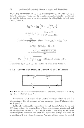
156. Continuous Models Using Ordinary Differential Equations 109
44. In a forest, the fox population grows at the rate of 10% per year and
the wolf population at the rate of 25% per year. The species compete
for the same resources and the forest can support 10000 foxes or 6000
wolves (carrying capacities).
(i) By taking F(t) and W(t) to be the fox and wolf populations at any
time t, formulate a mathematical model.
(ii) Find the solution for W(t) assuming W(0) = W0.
(iii) Assuming that the competition among the foxes and the wolves de-
creases the growth rates by an amount proportional to the product of
the two populations, modify the model to show the interaction of the
foxes and the wolves, 0.6 and 0.4 being the rates of decrease for the foxes
and the wolves respectively.
(iv) Find the equilibrium point(s) of the extended model obtained in
(iii).
(v) Perform linear stability analysis about the non-zero equilibrium
point and comment on the stability of the system.
(vi) Modify the model by considering an additional term to model the
hunting of both foxes and wolves, e being the measure of amount of hunt-
ing. At time t=0 (when hunting of both the species started), F(0)=1500
and W(0)=1000 and at time t=50, F(50)=100. Find the value of e for
this to happen.
(vii) Obtain the graph for long-term behavior of the two populations if
the level of hunting continues as in the previous question.
45. A model for interaction of messenger RNA-M and protein E is given by
dM
dt = Ek
1+Ek − αM and dE
dt = M − βE
(i) For k=1, interpret the model.
(ii) For k=1 and αβ 1, find the steady state(s) of the model.
(iii) Check for stability about the obtained steady state(s) and hence
obtain the phase plane diagram of the system.
(iv) Find the steady state solution(s) for k=2. What happens where
(a) αβ 1
2 (b) αβ = 1
2 and (c) αβ 1
2 ?
46. In biological pattern formation (zebra stripes and butterfly wing pat-
terns), Lewis [74] proposed a simple model involving a biochemical
switch, where a gene G is activated by a biochemical signal subsystem
S. The model is given by
dg
dt
= k1s0 − k2g +
k3g2
k2
4 + g2
where g(t) is the gene product concentration, the concentration s0 of S
is fixed and k
i s (i= 1,2,3,4) are positive constants.
(i) Describe the model and put it in the dimensionless form
dx
dτ
= s − rx +
x2
1 + x2

157. 110 Mathematical Modeling: Models, Analysis and Applications
by suitably determining dimensionless quantities.
(ii) Find the two fixed points for s=0. Is there any condition which needs
to be fulfilled? If yes, what is the condition?
(iii) If x(0) = 0, what happens to x(τ) if s is slowly increased from zero?
What happens if s then goes back to zero?
47. A particle moves in a plane with an acceleration
(i) which is always directed towards a fixed point and varies directly as
the distance from the fixed point.
(ii) which is always directed away from a fixed point and varies directly
as the distance from the fixed point.
If initially the particle is projected from the point (a,0) with a velocity V
along the y-axis (increasing direction), obtain the paths of the particle
for both cases.
48. A particle is projected vertically upwards with a speed u from a point
on the earth’s surface. Let v be the speed of the particle in any position
x, R be the radius of the earth, and g the acceleration due to gravity.
(i) Assuming that the acceleration due to gravity varies inversely as the
square of the distance x from the center of the earth and neglecting air
resistance, show that
v2
= u2
− 2gR2
1
R
−
1
x
(ii) If H is the greatest height reached by the particle, then show that
H =
2gR2
2gR − u2
− R.
49. The breadth of a river is L. O and A are two points on opposite sides of
the river bank such that OA is perpendicular to the direction of flow of
the river. A boat starts from point A to reach the other side and rows
with constant velocity u in such a manner that it is always directed
towards O. Show that the path of the boat is a parabola, assuming that
the river flows with the same velocity u.
50. A growth model of a population is given by
dN
dt
= aN2
− bN.
(i) Obtain the exact solution with N(0) = N0.
(ii) Explain how the growth rate depends on the population and sketch
the solution in the phase plane.
(iii) If N0 b
a , then show that N → ∞ and if N0 b
a , then N → 0.
What happens if N0 = b
a ?

158. Chapter 4
Spatial Models Using Partial
Differential Equations
4.1 Introduction ............................................................... 111
4.2 Different Mathematical Models Using Diffusion .......................... 112
4.2.1 Fluid Flow through a Porous Medium ........................... 112
4.2.2 Heat Flow through a Small Thin Rod (One Dimensional) ....... 113
4.2.3 Wave Equation .................................................... 115
4.2.4 Vibrating String .................................................. 117
4.2.5 Traffic Flow ....................................................... 119
4.2.6 Theory of Car-Following ......................................... 124
4.2.7 Crimes Model ..................................................... 125
4.3 Linear Stability Analysis .................................................. 127
4.3.1 One Species with Diffusion ........................................ 127
4.3.2 Two Species with Diffusion ...................................... 128
4.4 A Research Problem: Spatiotemporal Aspect of a Mathematical Model of
Cancer Immune Interaction Considering the Role of Antibodies .............. 131
4.4.1 Background of the Problem ....................................... 132
4.4.2 Spatiotemporal Model Formulation ............................... 132
4.4.3 Qualitative Analysis ............................................... 133
4.4.4 Numerical Results ................................................. 137
4.4.5 Conclusion ......................................................... 138
4.5 Miscellaneous Examples ................................................... 139
4.6 Exercises .................................................................. 148
4.1 Introduction
Real-world modeling depends on many variables simultaneously. So, when
we try to model some phenomena from the real world with the help of ordi-
nary differential equations (ODE), we restrict our analysis to one independent
variable (namely, time) only. That is, we only succeed in describing the dy-
namical behavior of the problem of interest with respect to that independent
variable. Thus, using ODE models means that we are considering that inde-
pendent variable, which is the most important factor affecting the problem of
interest, and other factors are taken to be negligible. Because of this restric-
tion, ODE models often fail to reflect the dynamics as shown by the acted
phenomena. Thus, a disparity between an ODE model and data may signify
that its state variables depend on more than one independent variable (say,
time and space). Hence, instead of using an ODE model in such cases, it may
be appropriate to use a partial differential equation (PDE) model.
111

159. 112 Mathematical Modeling: Models, Analysis and Applications
The advantage of PDE models are that they include derivatives of at least
two independent variables and hence we can describe the dynamical behavior
of our problem of interest in terms of two or more variables at the same
time. For example, if we consider the flow of heat in a metal bar, it would
be inappropriate NOT to model it with PDE to compute the temperature
distribution with respect to time as well as space (or distance in this case).
For example, we consider a simple predator-prey model (Lotka-Volterra)
dP1
dt
= α P1 − β P1P2
dP2
dt
= −γ P2 + δ P1P2
where we have used one independent variable (namely, time) to study the
dynamics of the system. But one can consider the effect of movement of the
prey and the predator, by adding a diffusion term to the equations, thereby
making it a PDE model. The equations
∂P1(x, t)
∂t
= α P1(x, t) − β P1(x, t)P2(x, t) + D1
∂2
P1(x, t)
∂x2
∂P2(x, t)
∂t
= −γ P2(x, t) + δ P1(x, t)P2(x, t) + D2
∂2
P2(x, t)
∂x2
are then able to capture the spatial aspect of the model and can give a com-
plete picture on the dynamics of the predator-prey system with respect to
both time and space.
4.2 Different Mathematical Models Using Diffusion
4.2.1 Fluid Flow through a Porous Medium
A porous medium is a material consisting of solid frame (also called matrix)
with pores. The pores, also known as voids, are interconnected and are filled
with liquid or gas or both.
To model the porous medium, we have to consider the three equations that
govern the flow:
(i) Equation of conservation of mass or continuity equation:
∂ρ
∂t
= −
−
→
∇.(ρ−
→
v ),
which states that the rate of mass entering a system is equal to the rate of
mass leaving the system.
(ii) Darcy’s law: v = −a
−
→
∇p, which states that velocity is proportional to
pressure gradient.

160. Spatial Models Using Partial Differential Equations 113
(iii) Equation of state: ρ = pγ
, where ρ is the fluid density, p is the pressure,
−
→
v is the flow velocity vector field and γ is a constant, which is the ratio of
specific heats.
The continuity equation gives
∂ρ
∂t
= −
−
→
∇.(ρ−
→
v )
=
−
→
∇.(ρa
−
→
∇p) (using (ii))
=
−
→
∇.(ρa
−
→
∇ρ1/γ
) (using (iii))
=
−
→
∇.
ρa
∂
∂x
î +
∂
∂y
ĵ +
∂
∂z
k̂
ρ1/γ
=
−
→
∇.
ρa
î
γ
ρ
1
γ −1 ∂ρ
∂x
+ ρa
ĵ
γ
ρ
1
γ −1 ∂ρ
∂y
+ ρa
k̂
γ
ρ
1
γ −1 ∂ρ
∂z
=
−
→
∇.(a
ρ1/γ
γ
−
→
∇ρ)
Now,
−
→
∇
ρ1+ 1
γ
=
î
∂
∂x
+ ĵ
∂
∂y
+ k̂
∂
∂z
ρ1+ 1
γ
=
1 +
1
γ
ρ
1
γ
−
→
∇ρ
Therefore,
∂ρ
∂t
=
−
→
∇.
⎛
⎝ a
−
→
∇ρ1+ 1
γ
γ
1 + 1
γ
⎞
⎠
=
a
1 + γ
∇2
ρ1+ 1
γ
Replacing ρ by u and rescaling t by a
1+γ , we get,
∂u
∂t
= um
where m = 1 + 1
γ and um
is the linear diffusion term with m 1. This
equation governs the flow of fluids through a porous media.
4.2.2 Heat Flow through a Small Thin Rod (One Dimen-
sional)
We consider a thin rod of length L, made of homogenous material (material
properties are translational invariant). We assume that the rod is perfectly

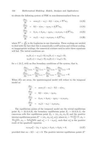
161. 114 Mathematical Modeling: Models, Analysis and Applications
FIGURE 4.1: A thin homogenous rod of length L, perfectly insulated along
its length.
insulated along its length so that heat can flow only through its ends (see
Figure 4.1).
Let u(x, t) be the temperature of this homogenous thin rod at a distance x
at time t. We consider an infinitesimal piece from the rod with length [x, x +
x]. If A is the cross-section of the rod and ρ is the density of the material
of the rod, then the infinitesimal volume is given by ΔV = AΔx and the
corresponding infinitesimal mass is Δm = ρAΔx. Then, the amount of heat
for the volume element is Q = σΔm u(x, t), where σ is the specific heat of
the material of the rod.
At time t + Δt, the amount of heat is
Q1 = σΔmu(x, t + Δt).
Change in heat = Q1 − Q = σΔm u(x, t + Δt) − σΔm u(x, t)
= σρA[u(x, t + Δt) − u(x, t)]Δx
Now, by the Fourier law of heat conduction, the heat flow is proportional to
the temperature gradient, that is, Q = −k ∂u
∂x = −kux(x, t) (in one dimen-
sion), where k is the thermal conductivity of the solid and the negative sign
denotes that the heat flux vector is in the direction of decreasing temperature.
Therefore, the change in heat must be equal to the heat flowing in at x, minus
the heat flowing out at x + Δx, during the time interval Δt, that is,
σρA[u(x, t + Δt) − u(x, t)]Δx = [−kux(x, t) − (−kux(x + Δt, t))]Δt
u(x, t + Δt) − u(x, t)
Δt
=
k
σρA
ux(x + Δx, t) − ux(x, t)
Δx
Taking Δx and Δt → 0, we get
∂u
∂t
= c2 ∂2
u
∂x2
,
which gives the required heat equation determining the heat flow through a
small thin rod. Here, c2
= k
σρA is called the constant thermal conductivity.
We use separation of variables to solve the above heat equation, which can
also be termed as a one dimensional diffusion equation.

162. Spatial Models Using Partial Differential Equations 115
Let u(x, t) = X(x) T (t) be a solution of ∂u
∂t = c2 ∂2
u
∂x2 . Substituting, we get,
X(x)T
(t) = c2
X
(x)T (t)
X
X
=
1
c2
T
T
= μ (a constant)
(Both functions must be equal to some constant as one of them is a function
of x only and the other is a function of t.)
⇒ X
= μX and T
= μc2
T, (4.1)
where μ is a separation constant.
Case I: μ is positive (= λ2
, say). From (4.1), we get X(x) = A1cosh (λx)+
A2sinh (λx) and T (t) = A3eλ2
c2
t
. Then, the solution of the heat equation is
u(x, t) = (C1cosh(λx) + C2sinh(λx))eλ2
c2
t
Case II: μ = 0. From (4.1), we get, X(x) = A4x + A5 and T (t) = A6.
Then, the solution of the heat equation is
u(x, t) = C3x + C4
Case III: μ is negative (= −λ2
, say). From (4.1), we get X(x) =
A7cos(λx) + A8sin(λx) and T (t) = A9e−λ2
c2
t
. Then, the solution of the heat
equation is
u(x, t) = (C5cos(λx) + C6sin(λx))e−λ2
c2
t
Combining, we can write the general solution of the heat equation as
u(x, t) =
⎧
⎨
⎩
(C1cosh(λx) + C2sinh(λx)) eλ2
c2
t
C3x + C4
(C5cos(λx) + C6sin(λx))e−λ2
c2
t
Note: (i) All three solutions are not consistent.
(ii) The first solution indicates t → ∞, u → ∞. So, it is reasonable to assume
that u(x, t) is bounded as t → ∞, from a realistic physical point of view.
(iii) The consistency of the third solution is always there, however, the second
solution is consistent in some cases along with the first.
4.2.3 Wave Equation
A homogeneous string of length L is tied at both ends. We assume that the
string offers no resistance due to bending, that is, it is thin and flexible; the
tension in the string is much greater than the gravitational force and hence
it can be neglected; the motion of the string takes place in the vertical plane
only (see Figure 4.2).

163. 116 Mathematical Modeling: Models, Analysis and Applications
FIGURE 4.2: A homogeneous string of length L, tied at both ends such that
the string offers no resistance due to bending.
Let ρ be the linear density of the string, and P and Q are two neighboring
points on the string such that arc PQ = Δs. Let T1 and T2 be the tensions at
points P and Q, which make angles α and β respectively with the x−axis and
u(x, t) be the displacement of the string at time t from its equilibrium state.
Then, the equations of motion are
T2cosβ − T1cosα = 0 (along x-axis) (4.2)
(ρΔS)
∂2
u
∂t2
= T2sinβ − T1sinα (along y-axis)
From (4.2), we get,
T1cosα = T2cosβ = T (say), which implies
(ρΔS)
T
∂2
u
∂t2
=
T2sinβ
T
−
T1sinα
T
=
T2sinβ
T2cosβ
−
T1sinα
T1cosα
⇒
(ρΔS)
T
∂2
u
∂t2
= tanβ − tanα
At the points P and Q, the slopes of the string are given by
tanα =
∂u
∂x
|x1 and tanβ =
∂u
∂x
|x2
Therefore
(ρΔS)
T
∂2
u
∂t2
= ux(x2, t) − ux(x1, t)
⇒
ρ
T
ΔS
Δx
∂2
u
∂t2
=
ux(x1 + Δx, t) − ux(x1, t)
Δx
As Δx → 0, Δs → Δx and we get
∂2
u
∂t2
= c2 ∂2
u
∂u2
, where c2
=
T
ρ
,
which is called the one-dimensional wave equation.

164. Spatial Models Using Partial Differential Equations 117
4.2.4 Vibrating String
We consider a homogenous flexible string of length L which is stretched
between two fixed points (0, 0) and (L, 0). Initially, the string is released from
a position u = f1(x) with a velocity ut = f2(x) parallel to the y−axis.
Mathematically, we can formulate the model as follows:
∂2
u
∂t2
= c2 ∂2
u
∂x2
; 0 ≤ x ≤ L; t 0
Boundary Conditions (BC): u(0, t) = 0 = u(L, t)
Initial Conditions (IC): u(x, 0) = f1(x), ∂u(x,0)
∂t = f2(x)
We use separation of variables to solve the given wave equation. Let
u(x, t) = X(x)T (t) be a solution of
∂2
u
∂t2
= c2 ∂2
u
∂x2
Substituting, we get,
X
X
=
T
c2T
= constant
Since the boundary conditions are periodic and homogenous in x, X(x) must
be periodic, which is only possible if the constant is negative = −λ2
(say).
Solving
X
X
= −λ2
and
T
c2T
= −λ2
, we get,
X(x) = A1cos(λx) + A2sin(λx) and T (t) = A3cos(cλt) + A4sin(cλt)
Therefore, the general solution is given by
u(x, t) = (A1cosλx + A2sinλx)(A3cos(cλt) + A4sin(cλt)) (4.3)
The boundary conditions u(0, t) = 0 = u(L, t) give
A1 = 0 and sin(λL) = 0 (A2 = 0)
⇒ λ = nπ
L , n being an integer.
Therefore equation (4.3) becomes
u(x, t) = A2sin
nπx
L
A3cos
cnπt
L
+ A4sin
cnπt
L
Noting that the wave equation is linear, we use the principle of superposition
to obtain its most general solution as
u(x, t) =
∞
n=1
Ancos
cnπt
L
+ Bnsin
cnπt
L
sin
nπx
L

165. 118 Mathematical Modeling: Models, Analysis and Applications
Using the initial condition we get,
u(x, 0) = f1(x) =
∞
n=1
Ansin
nπx
L
and
∂u(x, 0)
∂t
= f2(x) =
∞
n=1
cnπ
L
Bnsin
nπx
L
Both are half-range Fourier sine series, therefore we get,
An =
2
L
L
0
f1(x)sin
nπx
L
dx (4.4)
Bn =
L
nπc
2
L
L
0
f2(x)sin
nπx
L
dx (4.5)
Hence, the displacement of the vibrating string is given by
u(x, t) =
∞
n=1
Ancos
cnπt
L
+ Bnsin
cnπt
L
sin
nπx
L
where An and Bn are given by (4.4) and (4.5).
Corollary 1: If the homogenous flexible string of length L, stretched
between two fixed points (0, 0) and (L, 0) is initially released from rest from
a position u = f1(x), then its initial velocity is zero, that is, ∂u(x,0)
∂t = 0.
The solution in that case will be of the form
u(x, t) =
∞
n=1
Ancos
cnπt
L
sin
nπx
L
where
An =
2
L
L
0
f1(x)sin
nπx
L
dx
Corollary 2: If the homogenous flexible string of length L, stretched
between two fixed points (0, 0) and (L, 0) is initially released with velocity
f2(x), parallel to the axis of x from an equilibrium position (that is, y = 0),
then u(x, 0) = 0.
The solution in that case will be of the form
u(x, t) =
∞
n=1
Bnsin
cnπt
L
sin
nπx
L
where
Bn =
2
cnπ
L
0
f2(x)sin
nπx
L
dx

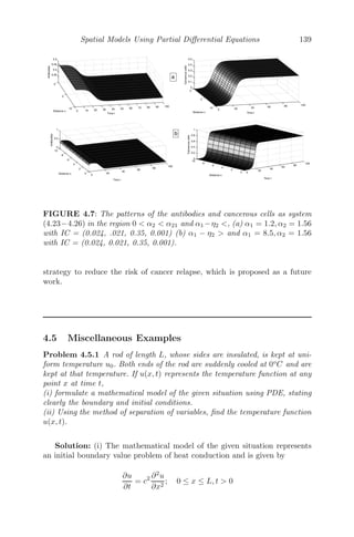
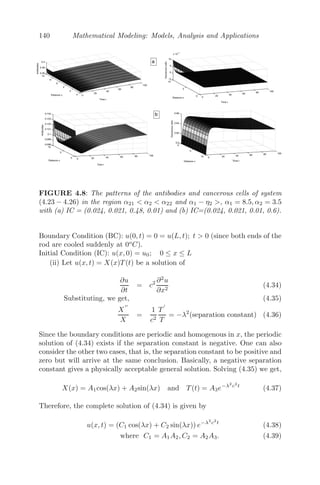
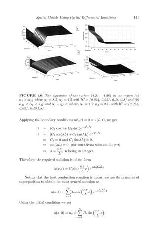
166. Spatial Models Using Partial Differential Equations 119
4.2.5 Traffic Flow
This section will concentrate on the macroscopic modeling of the traffic
flow, where the focus will be on modeling the density of cars and their flow,
rather than modeling individual cars and their velocity. Let the number of
cars per unit length at position x and in time t be ρ(x, t) and the number of
cars passing the position x per unit time at time t be f(x, t), that is, f(x, t)
gives the rate of flow of the cars (traffic flux) and ρ(x, t) denotes the density
of cars (the state variable).
We now use the global conservation law on the statement that ”cars are
conserved” [3]. By the statement ”cars are conserved,” we mean that the
number of cars in an arbitrary region of space I = [x1, x2], called the cell, at
the end of an arbitrary interval of time T = [t1, t2], called the time-step, is
equal to the number of cars in the cell at the beginning of the time-step (that
is, t), plus the number of cars entering the cell minus the number of cars going
out of the cell, that is, the change of flux in the cell [x1, x2].
Now, the number of cars entering the cell [x1, x2] through the point x1
during the time-step [t1, t2]
=
t2
t1
f(x1, t)dt
The number of cars leaving the cell [x1, x2] through the point x2 during the
time-step [t1, t2]
=
t2
t1
f(x2, t)dt
The number of cars in the cell [x1, x2] at time t1,
=
x2
x1
ρ(x, t1)dx
and the number of cars in the cell [x1, x2] at time t2
=
x2
x1
ρ(x, t2)dx
Since ”cars are conserved” we have
x2
x1
ρ(x, t2)dx =
x2
x1
ρ(x, t1)dx +
t2
t1
f(x1, t)dt −
t2
t1
f(x2, t)dt
⇒
x2
x1
[ρ(x, t2) − ρ(x, t1)]dx +
t2
t1
[f(x2, t) − f(x1, t)]dt = 0
Using the fundamental theorem of Calculus (by assuming ρ and f to be a

167. 120 Mathematical Modeling: Models, Analysis and Applications
smooth function of x and t respectively), we get,
x2
x1
t2
t1
∂ρ(x, t)
∂t
dtdx +
t2
t1
x2
x1
∂f(x, t)
∂x
dxdt = 0
⇒
x2
x1
t2
t1
∂ρ(x, t)
∂t
+
∂f(x, t)
∂x
dtdx = 0
(changing the order of integration for the second integral)
⇒
∂ρ(x, t)
∂t
+
∂f(x, t)
∂x
= 0 (4.6)
(assuming that the interval is piecewise continuous).
Now, suppose there are 50 cars per kilometer on a road and each car is
traveling at 80 km/h, then to a person standing at one side of the road, 80
km worth of cars will pass in one hour, that is, 50 × 80 = 4000 cars per hour.
In other words, the flux in this case is ρu = 50 cars/km×80 km/h
= 4000cars/h
Therefore, we can express traffic flux as a product of traffic density and ve-
locity, that is,
f(x, t) = ρ(x, t)u(x, t) (4.7)
Using (4.7), (4.6) becomes
∂ρ
∂t
+
∂(ρu)
∂x
= 0 (4.8)
Please note that the above continuity equation in one dimension has two
unknowns, namely, ρ and u, which are again functions of x and t. Since we
have only one partial differential equation, further information is necessary. A
reasonable assumption by a traffic modeler may be u = u(ρ), that is, velocity
of the car is a function of traffic density alone (such functions are called
equations of state or constitutive relations). Then (4.8) becomes
∂ρ
∂t
+
∂(ρu(ρ))
∂x
= 0
which is a partial differential equation of the first order.
Corollary 1: For a single lane open road, it is reasonable to take velocity
as a function of traffic density only. The simplest relation between car velocity
and traffic density is the linear relation
u(ρ) = umax
1 −
ρ
ρmax
, 0 ≤ ρ ≤ ρmax (4.9)
where umax is the maximum velocity with which an isolated car will travel,

168. Spatial Models Using Partial Differential Equations 121
either due to speed limits or condition of the road or driver caution, such that
u(0) = umax and ρmax is the maximum traffic density (bumper-to-bumper
traffic) where the velocity u is zero. Also, the velocity of the car diminishes
with traffic density and hence du
dρ 0, ρ 0, which is true for the function
(4.9).
Let g(ρ) = ρu(ρ) = umax
ρ −
ρ2
ρmax
, then (4.8) becomes
∂ρ
∂t
+
∂g(ρ)
∂x
= 0
⇒
∂ρ
∂t
+
dg
dρ
∂ρ
∂x
= 0
⇒
∂ρ
∂t
+ g
(ρ)
∂ρ
∂x
= 0 (4.10)
We next introduce a small perturbation in the traffic density ρ = ρ0 +
δρ(δρ ρ0), where ρ0 is a constant traffic density in (4.10). Then
g
(ρ) = g
(ρ0 + δρ) = g
(ρ0) + δρg
(ρ0) + .........
and the linearized form of (4.10) is
∂ρ
∂t
+ g
(ρ0)
∂ρ
∂x
= 0
The partial derivatives can be written as ∂
∂t (δρ) and ∂
∂x (δρ), but since both
the partial derivatives are of order δ, we have dropped δ from both terms.
Also, note that g
(ρ) = dg
dρ has the dimension of velocity, therefore g
(ρ0), also
having the dimension of velocity, is a constant, say, v0. Then the equation
becomes
∂ρ
∂t
+ v0
∂ρ
∂x
= 0 (4.11)
The general solution of (4.11) is given by
ρ = h(x − v0t)
which represents linear traffic waves and the velocity v0 is given by
v0 = umax
1 −
2ρ0
ρmax
We use the method of characteristics to solve (4.11). The characteristic base
curves for this problem are solutions of
dx
dt
= v0

169. 122 Mathematical Modeling: Models, Analysis and Applications
⇒ x = v0t + x0 (assuming x(0) = x0).
Clearly, this curve represents a straight line as both v0 and x0 are constants.
Let the initial traffic density be
ρ =
⎧
⎨
⎩
150 for x 0
150
1 − x0
2
, for 0 x 1
80, for x 1
ρmax = 1
4 cars per meter = 1000
4 = 250 cars per km and umax = 80 km/h.
Then, v0 = umax
1 −
2ρ0
ρmax
= 80
1 −
2 × 150
250
= −16km/h
for characteristics coming out of the negative x-axis and
v0 = 80
1 −
2 × 150
250
= 28.8km
for those emerging from x0 1. And for 0 x 1, we have
v0 = 80
1 −
2 × 150
1 − x
2
250
v0 = −16 + 48x0,
which shows a general transition.
Summarizing, we can say that since the traffic density ρ is constant for
each characteristic, we can calculate the traffic density in terms of x, for any
time. Thus, for x −16t, ρ = 150 and for x 1 + 28.8t, ρ = 80. In between
we can solve for x0 as
x = (−16 + 48x0)t + x0
x + 16t = (48t + 1)x0
x0 =
x + 16t
1 + 48t
Therefore, the traffic density for the in-between region is given by
ρ(x, t) = 150
1 −
x0
2
= 150
1 −
x + 16t
2(1 + 48t)
= 75
2 + 96t − x − 16t
1 + 48t
= 75
2 − x + 80t
1 + 48t

170. Spatial Models Using Partial Differential Equations 123
Corollary 2: We next consider an equation of the form [22]
∂ρ
∂t
+ v(ρ)
∂ρ
∂x
= 0, where v(ρ) =
√
ρ
and initial condition ρ(x, 0) = x, x 0
The characteristic base curves for this problem
dx
dt
= v(ρ(x(t), t)) =
ρ(x(t), t)
Though the problem looks complicated, note that ρ is constant on the charac-
teristic curve, implying v(ρ) =
ρ(x(t), t) is also constant and is independent
of t. Therefore,
x =
ρ(x(t), t) t + x0, since x(0) = x0
The function ρ is conserved along the characteristic base curves, which implies
ρ(x(t), t) = ρ(x(0), 0) = ρ(x0) = x0
⇒ x =
√
x0t + x0
(
√
x0)2
+ t
√
x0 − x = 0
x0 =
1
2
(t2
− t
t2 + 4x) + x
Therefore, the traffic density is obtained from
ρ(x0) = x0(x, t) as
ρ(x, t) =
1
2
(t2
− t
t2 + 4x) + x
Corollary 3: This method can be extended to non-homogenous initial
condition problems of the form
∂ρ
∂t
+ f(x, t)
∂ρ
∂x
= h(ρ, x, t)
The characteristic base curves for this problem are solutions of (as mentioned
earlier)
dx
dt
= f(x, t)
and
dρ
dt
= h(ρ, x, t)
is an arbitrary differential equation for ρ.

171. 124 Mathematical Modeling: Models, Analysis and Applications
4.2.6 Theory of Car-Following
There are various ways a modeler can model the response of a driver to
the surrounding traffic. One is the response of the driver and hence his car,
when another car is immediately in front of it, assuming that the car follows
a single lane with no passing (see Figure 4.3). A reasonable assumption would
be that the nth
car response to the (n + 1)th
car (which is immediately in
front of it) is proportional to their velocity difference (that is, velocity of the
(n + 1)th
car minus the velocity of the nth
car). Thus, if an is the acceleration
of the nth
car and un is its velocity, then [22],
FIGURE 4.3: Car follows single lane without passing, with another car im-
mediately in front of it.
an = λ(un+1 − un)
⇒ an = −λ(un − un+1)
⇒
d2
xn
dt2
= −λ
dxn
dt
−
dxn+1
dt
(4.12)
where xn is the position of the nth
car. Let the length of all the cars be L,
moving with the same speed u, at a distance D apart (equi-spaced).
Integrating (4.12) we get,
u =
dxn
dt
= −λ (xn − xn+1) + c,
c being the constant of integration. Therefore,
u = λ (xn+1 − xn) + c
= λ(L + D) + c
=
λ
ρ
+ c
where ρ = 1
L+D is the uniform car density.
Let the velocity u = 0, where ρ = ρmax, therefore c = − λ
ρmax
and
u(ρ) =
λ
ρ
−
λ
ρmax
,

172. Spatial Models Using Partial Differential Equations 125
which gives the velocity-density relation from the car-following theory. How-
ever, we observe that as ρ → 0, u → ∞ and hence we refine u(ρ) as follows:
u(ρ) =
umax, 0 ρ ρmin
λ
1
ρ − 1
ρmax
, ρmin ρ ρmax
where
umax = λ
1
ρ
−
1
ρmax
Let us now have a discussion with some numerical values for a more clear
picture. Let us assume that the driver of the nth
car will try to eliminate the
difference of the velocities in 10 seconds, that is, 1
10 th of the difference per
unit time, implying λ = 1
10 . Suppose the nth
and (n + 1)th
cars are moving at
a speed of 20 m/sec. Initially at t = 0, let the distance between the cars be
50 m, with car n at x = 0. At that exact moment, the (n + 1)th
car begins
constant deceleration, so that it stops in 10 seconds. then
un+1(t) = 20 − 2t (4.13)
Using (4.12) we get,
d2
xn
dt2
= −
1
10
dxn
dt
− (20 − 2t)
⇒
d2
xn
dt2
+
1
10
dxn
dt
=
(20 − 2t)
10
⇒ xn(t) = 40t − t2
+ 200(e−t/10
− 1)
where the initial conditions are
xn(0) = 0 and
dxn(0)
dt
= 20
Also, from (4.13), we get,
dxn+1(t)
dt
= 20 − 2t
xn+1(t) = 20t − t2
+ 50 (xn+1(0) = 50).
Clearly, the (n+1)th
car comes to a halt at time t = 10 seconds, at a distance
xn+1(10) = 150 m whereas
at t = 10,
dxn
dt
|t=10 = (40 − 2t − 20e−t/10
)t=10 = 12.64m/sec.
Thus, the nth
car have moved a distance of xn(10) = 173.576m and is still
moving. It will collide with the (n + 1)th
car after (50+150)−173.576
12.64 = 2.09
seconds.

173. 126 Mathematical Modeling: Models, Analysis and Applications
4.2.7 Crimes Model
Crimes occur in both urban and rural environments. Some areas are rea-
sonably safe while others are dangerous, demonstrating that crime is not uni-
formly distributed. Criminals have their favorite zones and victim types, who
are repeatedly targeted in a short time period [60, 61, 62, 64]. Some zones
are commonly known as crime hotspots [121, 130]. Crime patterns depend on
many factors. For example, the preference of a burglar to visit a previously
burglarized house or an adjacent one will depend on the information about
the schedules of the occupants or the types of valuables that may be stolen.
The preference of the burglar may also depend on the choice of some favor-
able neighborhood where past successful burglaries have created an impression
that the occupants are crime tolerant, resulting in the growth of more illegal
activities. This is known as the broken window effect [121, 133].
Here we discuss a simple crime model, namely residential burglary, which is
common in both urban and rural areas. The proposed model is a modification
of that given in [121]. Let A(x, y, t) denote the attractiveness to burglars and
C(x, y, t) be the criminal density for a location. The equations that model a
simple residential burglary are
∂A
∂t
= α CA − β A + D1∇2
A
∂C
∂t
= γ − δ CA + D2∇2
C, where, ∇2
≡
∂2
∂x2
+
∂2
∂y2
.
In the first equation, the term αCA shows the positive effect of successful
burglaries on attractiveness of location. A successful burglary at one location
encourages the burglars to repeat the crime at the same location or adjacent
to it. Thus, the density of burglars is increased due to attractiveness of a
location. The decay term (−βA) implies that with time, the attractiveness
of a particular location diminishes. Successful burglaries in the past may not
encourage the burglars to commit the crime more recently, resulting in the de-
cline of attractiveness of a location. The diffusion term D1∇2
A measures the
spread of attractiveness to the neighboring areas due to successful burglaries
in that location, D1( 0) being the diffusion coefficient.
In the second equation, γ is the constant source of burglars per area at a
given location. While some burglars leave the location after a successful bur-
glary, new thieves may enter the location due to its attractiveness and hence
a constant input of criminals is assumed. The term (−δCA) implicates that
due to the attractiveness of a location, a burglar will commit the burglary in
that location rather than moving to another one. Hence, there will be a reduc-
tion in the criminal density. The term D2∇2
C gives the random movement
of the criminals. Due to some unavoidable circumstances, a burglar may also
decide to move to a neighboring location, without committing a burglary in
the present location.

174. Spatial Models Using Partial Differential Equations 127
4.3 Linear Stability Analysis
4.3.1 One Species with Diffusion
We consider a one dimensional diffusion equation of the form
∂u(x, t)
∂t
= D
∂2
u(x, t)
∂x2
+ f(u) (4.14)
A homogenous steady state solution of this model is given by f(u0) = 0, as
the solution is constant in time and space, implying
∂u0
∂t
= 0 and
∂2
u0
∂x2
= 0 (4.15)
Let v(x, t) = u(x, t) − u0 be a small non-homogenous perturbation of the
homogenous steady state, then
∂v(x, t)
∂t
= D
∂2
v(x, t)
∂x2
+ f(u0 + v)
= D
∂2
v(x, t)
∂x2
+ f(u0) + vf
(u0) +
v2
2!
f
(u0) + ...
Using f(u0) = 0 and retaining linear terms, we get the linearized version of
(4.14) as
∂v(x, t)
∂t
= D
∂2
v(x, t)
∂x2
+ f
(u0)v(x, t) (4.16)
Let v(x, t) = Aeλt
cos(qx) be a solution of (4.16), then
Aeλt
cos(qx)[λ − f
(u0) + Dq2
] = 0
If A = 0, then the solution is trivial. For a non-trivial solution, we must have
λ = f
(u0) − Dq2
,
which gives the eigenvalue of the system, which is stable if
f
(u0) − Dq2
0
Note: For an ODE, u̇ = f(u), the system is stable if f
(u0) 0 and
unstable if f
(u0) 0. Thus, the diffusion will maintain stability in a stable
one-species system but it can stabilize an unstable one.

175. 128 Mathematical Modeling: Models, Analysis and Applications
4.3.2 Two Species with Diffusion
We consider a two species population with diffusion, given by
∂u1
∂t
= f1(u1, u2) + D1
∂2
u1
∂x2
∂u2
∂t
= f2(u1, u2) + D2
∂2
u2
∂x2
where f1(u1, u2) and f2(u1, u2) gives the interaction terms between two
species, which can be interspecific as well as intra specific, and D1 and D2 are
diffusion coefficients of first and second species respectively.
A spatially homogenous (uniform) steady state (u∗
1, u∗
2) of this model is
given by
f1(u∗
1, u∗
2) = 0, f2(u∗
1, u∗
2) = 0,
as the solution is constant in space and time implying
∂u∗
i
∂t
= 0 and
∂2
u∗
i
∂x2
= 0 (i = 1, 2)
Let
v1(x, t) = u1(x, t) − u∗
1
v2(x, t) = u2(x, t) − u∗
2
be small non-homogenous perturbations of the uniform steady state, then
∂v1
∂t
= f1(u∗
1 + v1, u∗
2 + v2) + D1
∂2
v1
∂x2
∂v2
∂t
= f2(u∗
1 + v1, u∗
2 + v2) + D2
∂2
v2
∂x2
Now,
∂v1
∂t
= f1(u∗
1 + v1, u∗
2 + v2) + D1
∂2
v1
∂x2
= D1
∂2
v1
∂x2
+ f1(u∗
1, u∗
2) + v1
∂f1
∂u1
|(u∗
1 ,u∗
2 ) + v2
∂f1
∂u2
|(u∗
1 ,u∗
2 )
+
v2
1
2!
∂2
f1
∂u2
1
(u∗
1 ,u∗
2 )
+ v1v2
∂2
f1
∂u1u2
(u∗
1 ,u∗
2)
+
v2
2
2!
∂2
f1
∂u2
2
(u∗
1 ,u∗
2 )
+ ...
Using f1(u∗
1, u∗
2) = 0 and retaining the linear terms, we get,
∂v1
∂t
= v1
∂f1
∂u1
(u∗
1 ,u∗
2 )
+ v2
∂f1
∂u2
(u∗
1 ,u∗
2 )
+ D1
∂2
v1
∂x2
(4.17)
In a similar manner we get,

176. Spatial Models Using Partial Differential Equations 129
∂v2
∂t
= v1
∂f2
∂u1
(u∗
1 ,u∗
2 )
+ v2
∂f2
∂u2
(u∗
1 ,u∗
2 )
+ D2
∂2
v2
∂x2
(4.18)
Let v1(x, t) = A1eλt
cos(qx) and v2(x, t) = A2eλt
cos(qx) be the solutions of
(4.17) and (4.18). Substituting v1 and v2 in (4.17) and (4.18) we get,
A1(λ − a11 + D1q2
) − A2a12 = 0
−a21A1 + (λ − a22 + D2q2
)A2 = 0
where
a11 =
∂f1
∂u1
(u∗
1 ,u∗
2)
, a12 =
∂f1
∂u2
(u∗
1 ,u∗
2)
, a21 =
∂f2
∂u1
(u∗
1 ,u∗
2)
,
a22 =
∂f2
∂u2
(u∗
1 ,u∗
2)
.
Clearly, A1 = 0, A2 = 0 is a solution, which is trivial and is dismissed as
we are interested in non-trivial solutions. Existence of a non-trivial solution
implies

180. λ − a11 + D1q2
−a12
−a21 λ − a22 + D2q2

184. = 0
⇒ λ2
−
−D2
1q2
− D2
2q2
+ a11 + a12
λ+(a11−D1q2
)(a22 −D2q2
)−a12a21 = 0
In the absence of diffusion, the characteristic equation is
⇒ λ2
− (a11 + a12) λ + (a11a22 − a12a21) = 0
The condition for stability is
a11 + a12 0 (4.19)
and a11a22 − a12a21 0 (4.20)
The conditions that the given system with diffusion have eigenvalues with
Reλ 0 are
a11 + a12 − (D1 + D2)q2
0 (4.21)
and (a11 − D1q2
)(a22 − D2q2
) − a12a21 0 (4.22)
However, diffusion may have a destabilizing effect on the system and violation
of any one of the conditions given by (4.21) or (4.22) will lead to diffusive
instability. Since D1, D2 and q2
are all positive quantities, (4.21) is always
true, provided (4.19) holds. Let
H(q2
) = (a11 − D1q2
)(a22 − D2q2
) − a12a21
= D1D2(q2
)2
− (D1a22 + D2a11)q2
+ (a11a22 − a12a21)

185. 130 Mathematical Modeling: Models, Analysis and Applications
FIGURE 4.4: The graph of H(q2
), which represents a parabola and geomet-
rically shows the region of diffusive instability.
Clearly, the condition for diffusive instability is H(q2
) 0. The graph of
H(q2
) is a parabola (as D1 0, D2 0) (see Figure 4.4) and the function
H(q2
) has a minimum. Putting dH(q2
)
dq2 = 0 and solving we get
q2
min =
1
2
a11
D1
+
a22
D2
Hence, the minimal condition for diffusive instability is
H(q2
min) 0
This implies
D1D2
4
a11
D1
+
a22
D2
2
− (D1a22 + D2a11)
1
2
a11
D1
+
a22
D2
+ (a11a22 − a12a21) 0
⇒ D1D2
(a11D2 + a22D1)2
D2
1D2
2
− 2
a11a22 +
a2
11D2
D1
+
a2
22D1
D2
+ a11a22
+ (a11a22 − a12a21) 0
⇒ D1D2
(a11D2 + a22D1)2
D2
1D2
2
− 2
(D1a22 + D2a11)2
D1D2
+ 4(a11a22 − a12a21) 0
⇒ (D1a22 + D2a11)2
4D1D2(a11a22 − a12a21)
⇒ (D1a22 + D2a11) 2
D1D2
√
a11a22 − a12a21
Summarizing the results, it is concluded that the conditions for diffusive in-
stability are
(i) a11 + a22 0.
(ii) a11a22 − a12a21 0.
(iii) (a11D2 + a22D1) 2
√
D1D2
√
a11a22 − a12a21.

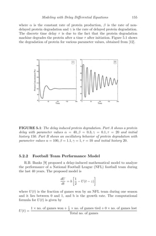
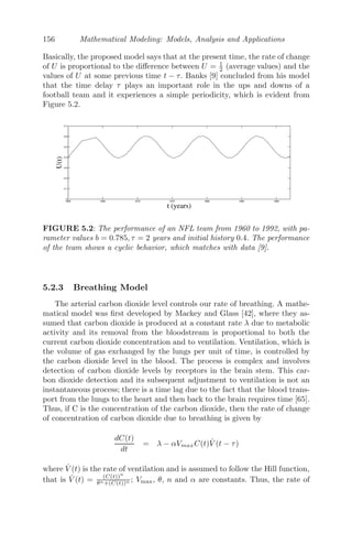
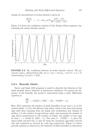
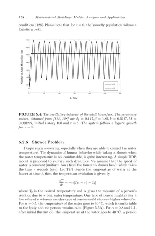
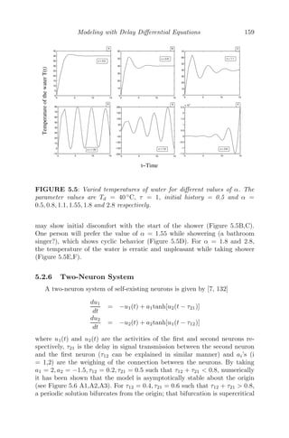
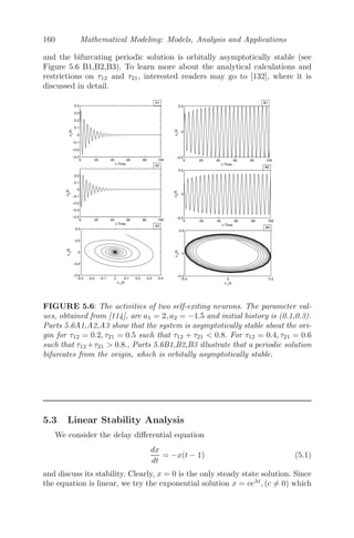
186. Spatial Models Using Partial Differential Equations 131
It is a well known fact that an equilibrium point which is asymptotically
stable in a non-spatial system may become unstable due to diffusion. Mathe-
matical analysis has confirmed that the diffusive system first attains instabil-
ity with respect to a spatially heterogeneous perturbation with a certain wave
number, which results in the formation of the so-called dissipative patterns or
regular spatial structure, known as Turing patterns.
Consider a prey-predator system (in dimensionless form) as
∂u
∂t
= u (1 − u) −
uv
u + α
+ ∇2
u
∂v
∂t
= β
uv
u + α
− γv + δ∇2
v,
where u(t,x,y) is the prey and v(t,x,y) is the predator. The prey population
follows a logistic growth, and declines due to consumption by the predator
population. The growth of the predator is directly proportional to the amount
of prey it has consumed and dies naturally, ∇2
u and δ∇2
v are diffusion terms,
which represent 2-dimensional movements, that is, ∇2
u ≡ ∂2
∂x2 + ∂2
∂y2 .
By taking α = 0.4, β = 2.0, γ = 0.6 and δ = 1, the system is solved
numerically by using MATLAB
code by Marcus R. Gurvie [36]. Figure 4.5
gives the spatial behavior of the prey and the predator respectively. It is
evident from the figure that there are irregular patches covering the whole
domain, a qualitative behavior which may be observed in plankton patterns
in the ocean [83].
(a) Prey density (b) Predator density
FIGURE 4.5: The spatial behavior of the prey and the predator. The param-
eter values are α = 0.4, β = 2.0, γ = 0.6, δ = 1, a = 0, b = 400, step-size h
= 1, maximum time T = 150 and the time-step = 1/3. The initial conditions
are u0(x, y) = 6./35 − 2 ∗ 10−7
∗ (X − 0.1 ∗ Y − 180).∗ (X − 0.1 ∗ Y − 800) and
v0(x, y) = 116./245 − 3 ∗ 10−5
∗ (X − 400) − 1.2 ∗ 10−4
∗ (Y − 150).

187. 132 Mathematical Modeling: Models, Analysis and Applications
4.4 A Research Problem: Spatiotemporal Aspect of a
Mathematical Model of Cancer Immune Interaction
Considering the Role of Antibodies
4.4.1 Background of the Problem
Mathematical modeling of tumor-immune system interaction has been
studied by many authors for the last four or five decades. These models have
a significant role in understanding the dynamics of the growth of cancerous
cells (or tumors) and their interaction with the host immune system for exper-
imentalists and clinicians. There is enough evidence that indicates the immune
system can recognize and eliminate malignant tumors [96, 124]. The focus is
now on how to enhance antitumor activity by stimulating the immune system
with vaccines or by direct injection of T-cells or cytokines [106, 107] or by
monoclonal antibody therapy [58]. Since the interaction strengths are density
dependent or concentration dependent, the interactions between tumor cells
and the other components of the tumor micro-environment are complex and
continuously changing. Hence, understanding these interactions sufficiently to
derive cancer immunotherapies has proven a very challenging task [34, 107].
Researchers have used mathematical models as a tool to investigate interac-
tions on different biological scales (e.g. molecular, cellular and tissue scales).
Mathematical models can also investigate the emergent properties of the sys-
tem, even though the properties of the individual components are not fully
known. These mathematical models are used to distill the essential compo-
nents of the interactions, thus identifying the most plausible mechanisms that
can lead to the observed outcomes. There is much existing literature, most
of which focus on non-spatial models, but several papers have begun to in-
vestigate the mathematical modeling of various aspects of the spatial features
associated with the immune response to cancer [18, 82, 86, 95, 99, 100].
Here, we propose a spatiotemporal mathematical model which describes
the interaction between the large B-cells, plasma cells, antibodies and the
cancerous cells using a system of non-linear partial differential equations. The
main interest here is the mathematical-modeling of antibody mediated im-
mune response to cancer, where various aspects of the dynamical behavior of
these complicated processes will be investigated. The interaction of the large
B-cells, plasma cells, antibodies with the cancerous cells is through diffusion.
4.4.2 Spatiotemporal Model Formulation
Large B-cells, plasma cells, antibodies and cancerous cells are heteroge-
neously distributed in the human physiological system. Taking into account
the diffusivity of large B-cells, plasma cells, antibodies and cancerous cells, the
governing equation for the interaction between then can be explained using a

188. Spatial Models Using Partial Differential Equations 133
system of partial differential equations. Let L, P, A and T be the number of
large B-cells, plasma cells, antibodies and cancerous cells at time t1. Then the
spatiotemporal mathematical model for the interaction of the cancerous cells
and the host immune system is given by
∂L
∂t1
= a1uL(1 −
L
K1
) − b1(1 − u)L + D1∇2
L,
∂P
∂t1
= b1(1 − u)L − μ1P + D2∇2
P,
∂A
∂t1
= r1L + r2P − μ2A − β1AT + D3∇2
A,
∂T
∂t1
= rT (1 −
T
K2
) − β2AT + D4∇2
T,
The large B-cells proliferate at a constant growth rate a1 following a logistic
growth, and differentiate into plasma cells at the constant rate b1. K1 is the
carrying capacity of the large B-cells, u is the fraction of the population of large
B-cells which remains as the proliferating population, and (1-u) is the fraction
of the large B-cell population which differentiate into plasma cells. μ1 and μ2
are the natural death rates of the plasma cells and the antibodies respectively
and r1 and r2 are the rates at which the large B-cells and the plasma cells
secrete antibodies respectively. The intrinsic growth rate of the cancerous cells
is denoted by r and its carrying capacity by K2. β1 and β2 are the constant
rates of loss of the antibodies and the cancerous cells respectively due to
interaction between them. D
is (i = 1, 2, 3, 4), are constant positive diffusion
coefficients of the large B-cells, plasma cells, antibodies and the cancerous
cells respectively and ∇2
= ∂2
∂X2 is the Laplacian in one dimension. The initial
conditions L(0, X) = L0, P(0, X) = P0, A(0, X) = A0, T (0, X) = T0, forX ∈
[0, l], are assumed to be positive functions and we assume no flux boundary
conditions of the system, that is,
∂L
∂X
|(t,0) =
∂L
∂X
|(t,l) =
∂P
∂X
|(t,0) =
∂p
∂X
|(t,l) = 0
∂A
∂X
|(t,0) =
∂A
∂X
|(t,l) =
∂T
∂X
|(t,0) =
∂T
∂X
|(t,l) = 0.
4.4.3 Qualitative Analysis
To reduce the number of system parameters, the spatiotemporal model
can be written in dimensionless variables using the following scaling:
w1 =
L
K1
, w2 =
P
K1
, w3 =
A
K2
, w4 =
T
K2
, t = rt1, X = λx,
λ2
=
D1
r
, d2 =
D2
D1
, d3 =
D3
D1
, d4 =
D4
D1
, a =
a1
r
, b =
b1
r
, η1 =
μ1
r
,
η2 =
μ2
r
, k1 =
r1K1
rK2
, k2 =
r2K1
rK2
, α1 =
β1K2
r
, α2 =
β2K2
r
,

189. 134 Mathematical Modeling: Models, Analysis and Applications
to obtain the following system of PDE in non-dimensionalized form as
∂w1
∂t
= auw1(1 − w1) − b(1 − u)w1 + ∇2
w1, (4.23)
∂w2
∂t
= b(1 − u)w1 − η1w2 + d2∇2
w2, (4.24)
∂w3
∂t
= k1w1 + k2w2 − η2w3 − α1w3w4 + d3∇2
w3, (4.25)
∂w4
∂t
= w4(1 − w4) − α2w3w4 + d4∇2
w4, (4.26)
where ∇2
= ∂2
∂x2 is the Laplacian in one dimension. These scalings are needed
to deal with the fact that this is numerically a stiff system and without scaling,
or inappropriate scalings, the numerical routines used to solve these equations
will fail. The initial conditions are
w1(0, x) = w10( 0); w2(0, x) = w20( 0);
w3(0, x) = w30( 0); w4(0, x) = w40( 0),
for x ∈ [0, l], with no flux boundary conditions of the system, that is,
∂w1
∂x
|(t,0) =
∂w1
∂x
|(t,l) =
∂w2
∂x
|(t,0) =
∂w2
∂x
|(t,l) = 0
∂w3
∂x
|(t,0) =
∂w3
∂x
|(t,l) =
∂w4
∂x
|(t,0) =
∂w4
∂x
|(t,l) = 0.
When D
is are zeros, the spatiotemporal model will reduce to the temporal
model as:
dw1
dt
= auw1(1 − w1) − b(1 − u)w1,
dw2
dt
= b(1 − u)w1 − η1w2,
dw3
dt
= k1w1 + k2w2 − η2w3 − α1w3w4,
dw4
dt
= w4(1 − w4) − α2w3w4.
The equilibrium points of the temporal model are the trivial equilibrium
point E0 = (0, 0, 0, 0), the boundary equilibrium point E1 = (0, 0, 0, 1), the
cancerous cells free equilibrium point E2 = (w̄1, w̄2, w̄3, 0) and the positive
interior equilibrium points E∗
= (w̄1, w̄2, w∗
3, w∗
4), where w̄1 = au−b(1−u)
au , w̄2 =
b(1−u)w̄1
η1
, w̄3 = k1w̄1+k2w̄2
η2
and w∗
4 = 1 − α2w∗
3, such that w∗
3 is the positive
roots of the quadratic equation
α1α2w2
3 − (α1 + η2)w3 + k2w̄1 + k2w̄2 = 0, (4.27)
provided that au − b(1 − u) 0. The positive interior equilibrium points E∗

190. Spatial Models Using Partial Differential Equations 135
exist if the cancerous cells free equilibrium point exists, the quadratic equa-
tion (4.27) has positive real roots and 1 − α2w∗
3 0. The quadratic equation
(4.27) has positive real roots if α2 (α1+η2)2
4α1(k1w̄1+k2w̄2) = α22 (say). There-
fore, both the positive interior equilibrium points E∗
+ = (w̄1, w̄2, w∗
3+, w∗
4+),
which is characterized by a relatively low number of cancerous cells and E∗
− =
(w̄1, w̄2, w∗
3−, w∗
4−), characterized by a relatively high number of cancerous
cells exist if 1
w̄3
α2 (α1+η2)2
4α1(k1w̄1+k2w̄2) and α1 − η2 0. If 0 α2 1
w̄3
= α21
(say), then from the positive interior equilibrium points only the high number
of cancerous cells equilibrium point E∗
− exists.
0 5 10 15
0
1
2
3
4
5
6
α
1
α
2
RI
α
2
=α
21
=η
2
/k
α
1
=η2
α
2
=α
22
=(α
1
+η
2
)
2
/(4kα
1
)
R
I
R
II
R
III
RIV
FIGURE 4.6: The existence regions of the equilibrium points E2, E∗
+ and
E∗
−, where k = k1x̄ + k2ȳ. RI (α1 − η2 0 and 0 α2 α21 = 2.08591) is
the region where E2 and E∗
− exist. RII (α1 − η2 0 and α21 α2 α22)
is the region where the equilibrium points E2 and E∗
− and E∗
+ exist. RIII
(α2 α22) is the region where the equilibrium point E2 only exists. In the
region RIV (α1 − η2 0 and α21 α2 α22), the equilibrium point E2 only
exists.
From the linear stability analysis of the temporal model one can easily
show that
(i) The trivial equilibrium point E0 is unstable always and the boundary equi-
librium point E1 is locally asymptotically stable if au − b(1 − u) 0.
(ii) The cancerous cells free equilibrium point E2 is locally asymptotically
stable if 1 − α2w̄3 0 and the positive interior equilibrium point E∗
−, which
is characterized by relatively high number of cancerous cells, is locally asymp-
totically stable when it exists.
(iii) The positive interior equilibrium point E∗
+, with relatively cancerous cells

191. 136 Mathematical Modeling: Models, Analysis and Applications
is unstable when it exists.
Figure 4.6 gives the regions of existence of the equilibrium points with
respect to the parameters α1 and α2.
The positive interior equilibrium point E∗
− = (w̄1, w̄2, w∗
3−, w∗
4−), which
is locally asymptotically stable in the temporal system, when it exists, is a
spatially homogeneous steady state for the reaction diffusion equations (4.23−
4.26). Diffusion driven instability occurs when a temporally stable equilibrium
point becomes unstable because of the diffusive property of the interacting
populations [129]. To study the effect of diffusion on the temporal system, we
slightly perturb the temporally stable equilibrium point E∗
− and observe how
the small perturbation of the homogeneous equilibrium point develops in the
large time limit. For this, we consider the following perturbation
u1(x, t) = w̄1 + C1 cos kx,
u2(x, t) = w̄2 + C2 cos kx,
u3(x, t) = w3− + C3 cos kx,
u4(x, t) = w4− + C4 cos kx,
⎫
⎪
⎪
⎪
⎬
⎪
⎪
⎪
⎭
(4.28)
where Ci (i = 1, 2, 3, 4), are positive constants and k is the wave number.
Substituting the above equation in (4.23−4.26), we linearize the system about
the positive interior equilibrium point E∗
− to obtain the following system of
PDEs:
∂u1
∂t
= −(au − b(1 − u))u1 −
∂2
u1
∂x2
, (4.29)
∂u2
∂t
= b(1 − u)u1 − η1u2 − d2
∂2
u2
∂x2
, (4.30)
∂u3
∂t
= k1u1 + k2u2 − (η2 + α1w∗
4)u3 − α1w∗
3u4 − d3
∂2
u3
∂x2
, (4.31)
∂u4
∂t
= −α2w∗
4u3 + (1 − 2w∗
4 − α2w∗
3)u4 − d4
∂2
u4
∂x2
. (4.32)
The corresponding Jacobian matrix JE∗
−
at the positive interior equilibrium
point E∗
− is given by
JE∗
−
=
⎛
⎜
⎜
⎝
−q0 − k2
0 0 0
b(1 − u) −η1 − d2k2
0 0
k1 k2 −(η2 + α1w∗
4 + d3k2
) −α1w∗
3
0 0 −α2w∗
4 −(w∗
4 + d4k2
)
⎞
⎟
⎟
⎠
and the corresponding characteristic equation is given by
(λ + au − b(1 − u) + k2
)(λ + η1 + d2k2
) × [λ2
+ (η2 + (1 + α1)w∗
4 + (d3 + d4)k2
)λ
+(d3 + d4)k4
+ (w∗
4 + (η2 + α1w∗
4)d4)k2
+ w∗
4(η2 + α1 − 2α1α2w∗
3)] = 0

192. Spatial Models Using Partial Differential Equations 137
From the existence of the cancerous cells free equilibrium point, we know that
au − b(1 − u) 0. Hence the linear stability analysis of the spatiotemporal
model depends on the solution of the quadratic equation:
0 = λ2
+ (η2 + (1 + α1)w∗
4 + (1 + d4)k2
)λ (4.33)
+ (w∗
4 + (η2 + α1w∗
4)d4)k2
+ d4k4
+ w∗
4(η2 + α1 − 2α1α2w∗
3).
But, from (4.29) and (4.33), we have
η2 + α1 − 2α1α2w∗
3 =
(α1 + η2)2 − 4α1α2(k1w̄1 + k2w̄2),
which is positive at the positive interior equilibrium point E∗
−. Hence λ is
negative or complex with negative real part, since α1, η2, d4, k2
and w∗
4 are all
positive. Therefore, the equilibrium point E∗
− is always spatially stable. One
can easily check that the tumor free equilibrium point is also spatially stable
(always).
4.4.4 Numerical Results
The system is solved numerically with respect to time and space con-
sidering the positive initial conditions (w1(0, x) = w10 0, w2(0, x) = w20
0, w3(0, x) = w30 0, w4(0, x) = w40 0, for x ∈ [0, l]) with no flux boundary
conditions. From the stability analysis of the reaction diffusion equations, the
temporally stable positive interior equilibrium point E∗
− remains stable due to
a small spatiotemporal perturbation. The dynamics of the system about the
equilibrium point E∗
− is the only point for discussion here as all other points
are irrelevant from a biological point of view when the spatial aspect has been
considered. The parameter values used for numerical simulations and their
sources are listed in tabular form (Table 4.1).
In the parametric region R1 : 0 α2 α21, the high number of the
cancerous cells equilibrium point E∗
− is the only locally asymptotically stable
equilibrium point of the system. In this region, the cancerous cells are able
to overcome the immune system surveillance, that is, they survive. Figure 4.7
shows the dynamics of the system in this region.
In the region R2 : α21 α2 α22 (α1 − η2 0), both the cancer free cells
and the high number of cancerous cell equilibrium points are locally asymp-
totically stable, that is, it is a region of bi-stability. In this region the system
is highly sensitive to the initial condition and some of the values of the sys-
tem parameters. A slight change in the initial conditions around the region
of attraction of this equilibrium point causes a drastic change in the behav-
ior of the system in this region. The cancer burden may reduce (first panel)
or increase (second panel) depending on initiation of the therapy (such as,
monoclonal antibody therapy) which may be capable of changing the system

193. 138 Mathematical Modeling: Models, Analysis and Applications
TABLE 4.1: Parameter Values
Parameters Values Scaled References
a1 (0.02 − 0.2) hr.−1
0.0464 -0.464 [97]
b1 0.01 hr.−1
0.0232 [97]
μ1 (0.002 − 0.02) hr.−1
0.00464-
0.0464
[97]
K1 1.25 × 107
cells − [97]
u 0.1 − [97]
r1 100 Ab cell−1
sec.−1
2.95942 [84]
r2 1000 Ab cell−1
sec.−1
29.5942 [84]
μ2 0.1277 − 0.6465 hr.−1
0.2963 - 1.5 [31]
β1 4.5 × 10−10
− 2.5448 ×
10−6
cell−1
hr.−1
1.0232 -
5786.32
[31]
r 0.431 day−1
− [100]
K2 9.8 × 108
cells − [100]
β2 6.6 × 10−10
− 2.4935 ×
10−7
Ab−1
hr.−1
1.5 −
566.968
[31]
parameters. The dynamics of the system are depicted in Figure 4.8.
In the regions R3 : α2 α22 and R4 : α21 α2 α22, α1 − η2 0,
the cancerous cells free equilibrium point is the only equilibrium point of the
system which is locally asymptotically stable. In these regions, the antibodies
are able to successfully eradicate the cancerous cells. Any amount of cancerous
cells are eradicated with time. This situation is depicted in Figure 4.9.
4.4.5 Conclusion
In this example, we have examined a spatiotemporal mathematical model
describing the interaction of cancerous cells in the presence of humoral (anti-
body) mediated immune response. In particular, we have focused our attention
upon the interaction of cancer cells with antibodies through diffusion. Ana-
lytical study shows that the system always remains stable when the spatial
aspect is taken into account. Numerically, it is shown that for a particular
choice of parameters, the model was able to simulate the phenomenon of can-
cer dormancy - a clinical condition that has been observed in colon cancer,
breast cancer and in several types of lymphomas. The model also allows us
to identify certain critical system parameters, that can reduce cancer burden.
However, there are few significant features which may not be included in this
model. For example, a bifurcation analysis of the spatiotemporal model can
give a better understanding of the system parameters that may lead to cancer
dormancy and cancer regrowth mechanisms and in optimizing the therapeutic

194. Spatial Models Using Partial Differential Equations 139
0
5
10
0 10 20 30 40 50 60 70 80 90 100
0.35
0.4
0.45
0.5
Time t
Distance x
Antibodies
0
5
10
0 20 40 60 80 100
0
0.1
0.2
0.3
0.4
0.5
Time t
Distance x
Cancerous
cells
0
2
4
6
8
10
0
20
40
60
80
100
0
0.5
1
Time t
Distance x
Antibodies
0
2
4
6
8
10
0
20
40
60
80
100
0
0.2
0.4
0.6
0.8
1
Time t
Distance x
Cancerous
cells
a
b
FIGURE 4.7: The patterns of the antibodies and cancerous cells as system
(4.23−4.26) in the region 0 α2 α21 and α1 −η2 , (a) α1 = 1.2, α2 = 1.56
with IC = (0.024, .021, 0.35, 0.001) (b) α1 − η2 and α1 = 8.5, α2 = 1.56
with IC = (0.024, 0.021, 0.35, 0.001).
strategy to reduce the risk of cancer relapse, which is proposed as a future
work.
4.5 Miscellaneous Examples
Problem 4.5.1 A rod of length L, whose sides are insulated, is kept at uni-
form temperature u0. Both ends of the rod are suddenly cooled at 0o
C and are
kept at that temperature. If u(x, t) represents the temperature function at any
point x at time t,
(i) formulate a mathematical model of the given situation using PDE, stating
clearly the boundary and initial conditions.
(ii) Using the method of separation of variables, find the temperature function
u(x, t).
Solution: (i) The mathematical model of the given situation represents
an initial boundary value problem of heat conduction and is given by
∂u
∂t
= c2 ∂2
u
∂x2
; 0 ≤ x ≤ L, t 0

195. 140 Mathematical Modeling: Models, Analysis and Applications
0
2
4
6
8
10
0
20
40
60
80
100
0.46
0.48
0.5
Time t
Distance x
Antibodies
0
5
10
0 20 40 60 80 100
−5
0
5
10
x 10
−4
Time t
Distance x
Cancerous
cells
0
5
10
0 20 40 60 80 100
0.098
0.099
0.1
0.101
0.102
0.103
0.104
Time t
Distance x
Antibodies
0
5
10 0 20 40 60 80 100
0.6
0.62
0.64
0.66
Time t
Distance x
Cancerous
cells
a
b
FIGURE 4.8: The patterns of the antibodies and cancerous cells of system
(4.23 − 4.26) in the region α21 α2 α22 and α1 − η2 , α1 = 8.5, α2 = 3.5
with (a) IC = (0.024, 0.021, 0.48, 0.01) and (b) IC=(0.024, 0.021, 0.01, 0.6).
Boundary Condition (BC): u(0, t) = 0 = u(L, t); t 0 (since both ends of the
rod are cooled suddenly at 0o
C).
Initial Condition (IC): u(x, 0) = u0; 0 ≤ x ≤ L
(ii) Let u(x, t) = X(x)T (t) be a solution of
∂u
∂t
= c2 ∂2
u
∂x2
(4.34)
Substituting, we get, (4.35)
X
X
=
1
c2
T
T
= −λ2
(separation constant) (4.36)
Since the boundary conditions are periodic and homogenous in x, the periodic
solution of (4.34) exists if the separation constant is negative. One can also
consider the other two cases, that is, the separation constant to be positive and
zero but will arrive at the same conclusion. Basically, a negative separation
constant gives a physically acceptable general solution. Solving (4.35) we get,
X(x) = A1cos(λx) + A2sin(λx) and T (t) = A3e−λ2
c2
t
(4.37)
Therefore, the complete solution of (4.34) is given by
u(x, t) = (C1 cos(λx) + C2 sin(λx)) e−λ2
c2
t
(4.38)
where C1 = A1A2, C2 = A2A3. (4.39)

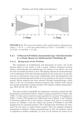
196. Spatial Models Using Partial Differential Equations 141
0
2
4
6
8
10
0 20 40 60 80 100
0.1
0.2
0.3
0.4
0.5
Time t
Distance x
Antibodies
0
5
10
0 10 20 30 40 50 60 70 80 90 100
−0.2
0
0.2
0.4
0.6
0.8
Time t
Distance x
Cancerous
cells
0
5
10
0
20
40
60
80
100
0.35
0.4
0.45
0.5
Time t
Distance x
Antibodies
0
5
10
0
20
40
60
80
100
0
0.2
0.4
0.6
0.8
Time t
Distance x
Cancerous
cells
a
b
FIGURE 4.9: The dynamics of the system (4.23 − 4.26) in the region (a)
α2 α22 where α1 = 8.5, α2 = 4.5 with IC = (0.024, 0.021, 0.48, 0.8) and (b)
α21 α2 α22 and α1 − η2 where, α1 = 1.2, α2 = 2.1, with IC = (0.024,
0.021, 0.48,0.8).
Applying the boundary conditions u(0, t) = 0 = u(L, t), we get
0 = (C1 cos 0 + C2 sin 0)e−λ2
c2
t
0 = [C1 cos(λL) + C2 sin(λL)]e−λ2
c2
t
⇒ C1 = 0 and C2 sin(λL) = 0.
⇒ sin(λL) = 0 (for non-trivial solution C2 = 0)
⇒ λ =
nπ
L
, n being an integer.
Therefore, the required solution is of the form
u(x, t) = C2sin
nπ
L
x
e
−n2π2c2
L t
Noting that the heat conduction equation is linear, we use the principle of
superposition to obtain its most general solution as
u(x, t) =
∞
n=1
Bnsin
nπ
L
x
e
−n2π2c2
L t
Using the initial condition we get
u(x, 0) = u0 =
∞
n=1
Bnsin
nπ
L
x

197. 142 Mathematical Modeling: Models, Analysis and Applications
which is a half-range Fourier series, where
Bn =
2
L
L
0
u0 sin
nπ
L
x
dx
=
2u0
nπ
(1 − cosnπ)
=
2u0
nπ
[1 − (−1)n
]
Therefore,
Bn =
4u0
nπ , nis odd
0, n is even
In general, we can write
Bn =
4u0
(2n + 1)π
, n = 0, 1, 2, ...
Hence, the temperature function is given by
u(x, t) =
∞
n=1
4u0
(2n + 1)π
sin
nπx
L
e
−n2π2c2
L t
Problem 4.5.2 A rod of length 10 cm, whose sides are insulated, is kept at
temperature 0 ◦
C and 100 ◦
C at its ends A and B respectively, until the steady
state condition prevails. The temperature at end A is suddenly increased to
20 ◦
C and at end B, it is decreased to 60 ◦
C. Formulate a mathematical model
of the given situation and obtain the temperature function at any time t.
Solution:
PDE :
∂u
∂t
= c2 ∂2
u
∂x2
, 0 ≤ x ≤ 10;
BC : u(0, t) = 0, u(10, t) = 100.
Before the temperature at the ends of the rod are changed, the heat flow in
the rod is independent of time when steady state is reached. Therefore, at the
steady state
d2
u
dx2
= 0 ⇒ us(x) = C1x + C2
Applying boundary conditions we get, C1 = 10, C2 = 0. Thus, the initial
steady temperature distribution in the rod is
us(x) = 10x
In a similar manner, when the temperature at the ends of the rod are changed
to 20 ◦
C and 60 ◦
C respectively, the final steady temperature in the rod is
us(x) = 4x + 20,

198. Spatial Models Using Partial Differential Equations 143
which will happen after a long time (several hours).
To obtain the temperature distribution u(x, t) in the intermediate period,
we write
u(x, t) = us(x) + u1(x, t)
when u1(x, t) → 0 as t → ∞ and is called the transient temperature dis-
tribution, which satisfies the PDE. Therefore, the general solution is given
by
u(x, t) = (4x + 20) + e−c2
λ2
t
(A1cosλx + A2sinλx)
Using the boundary conditions
u(0, t) = 20 and u(10, t) = 60 we get,
20 = 20 + A1e−c2
λ2
t
⇒ A1 = 0
60 = 60 + A2 sin(10λ)e−c2
λ2
t
⇒ sin(10λ) = 0 (since A2 = 0 for non-trivial solution)
⇒ λ =
nπ
10
.
Using the superposition principle, we get,
u(x, t) = (4x + 20) +
∞
n=1
Bnsin
nπx
10
e
−c2n2π2
100 t
Using the initial condition u(x, 0) = 10x gives
10x = 4x + 20 +
∞
n=1
Bnsin
nπx
10
6x − 20 =
∞
n=1
Bnsin
nπx
10
where Bn =
2
10
10
0
(6x − 10)sin
nπx
10
dx =
1
5
(−1)n 800
nπ
−
200
nπ
Problem 4.5.3 A homogenous flexible string in a guitar is stretched between
two fixed points (0, 0) and (2, 0), the length of the string being 2 units. The
string of the guitar is initially plucked from rest from a position sin3
πx
2
.
Find the displacement u(x, t) of the string of the guitar at time t.
Solution: Assuming that the string of the guitar is pulled aside and re-
leased, mathematically, the model can be formulated as follows:
∂2
u
∂t2
= c2 ∂2
u
∂x2
, 0 ≤ x ≤ L; t 0
Boundary conditions (BC): u(0, t) = 0 = u(2, t)
Initial conditions (IC): u(x, 0) = sin3
πx
2
, ∂u(x,0)
∂t = 0.
The physically acceptable solution is of the form
u(x, t) = (A1cosλx + A2sinλx)(A3cos(cλt) + A4sin(cλt))

199. 144 Mathematical Modeling: Models, Analysis and Applications
Applying boundary conditions we get A1 = 0 and A2sin(2) = 0 ⇒ λ =
nπ
2 (A2 = 0, )n = 1, 2, ... Also, ∂u(x,0)
∂t = 0 ⇒ A4 = 0. Using the principle of
superposition, the possible solution is given by
u(x, t) =
∞
n=1
Ansin
nπx
2
cos
cπnt
2
Using the initial condition u(x, 0) = sin3
πx
2
, we get,
sin3
πx
2
=
∞
n=1
Ansin
nπx
2
⇒
3
4
sin
πx
2
−
1
4
sin
3πx
2
= A1sin
πx
2
+ A2sin
2πx
2
+ A3sin
3πx
2
+ A4sin
4πx
2
+ ...
Comparing, we get,
A1 =
3
4
and A3 = −
1
4
,
while all other A
is are zeros. Therefore, the required solution is
u(x, t) =
3
4
sin
πx
2
cos
πct
2
−
1
4
sin
3πx
2
cos
3πct
2
Problem 4.5.4 A homogenous flexible string in a guitar is stretched between
two fixed points (0, 0) and (L, 0), the length of the string being L units. The
string of the guitar is initially plucked from rest from a position μx(L − x).
Find the displacement u(x, t) of the string of the guitar at time t.
Solution:
∂2
u
∂t2
= c2 ∂2
u
∂x2
, 0 ≤ x ≤ L; t 0
Boundary conditions (BC): u(0, t) = 0 = u(L, t). Initial conditions (IC):
u(x, 0) = μx(L − x), ∂u(x,0)
∂t = 0. The solution is of the form
u(x, t) = (A1cosλx + A2sinλx)(A3cos(cλt) + A4sin(cλt))
Applying boundary conditions we get A1 = 0, λ = nπ
2 (A2 = 0, ), n being an
integer. Using the principle of superposition, the possible solution is
u(x, t) =
∞
n=1
Ancos
cnπt
L
+ Bnsin
cnπt
L
sin
nπx
L
Now, ∂u(x,0)
∂t = 0 gives Bn = 0
⇒ u(x, t) =
∞
n=1
Ancos
cnπt
L
sin
nπx
L

200. Spatial Models Using Partial Differential Equations 145
The last initial condition gives
u(x, 0) = μx(L − x) =
∞
n=1
Ansin
nπx
L
,
which is a half-range Fourier sine series, where
An =
2
L
L
0
μx(L − x)sin
nπx
L
dx
=
2μ
L
2
L
nπ
3
{1 − (−1)n
}
=
8μL2
n3π3 ; n = odd
0; n = even
Therefore, the required solution is
u(x, t) =
∞
n=1
8μL2
(2n − 1)3π3
cos
(2n − 1)cπt
L
sin
(2n − 1)πx
L
.
Problem 4.5.5 Find the traffic density ρ(x, t), satisfying
∂ρ
∂t
+ (xsint)
∂ρ
∂x
= 0
with initial condition ρ0(x) = 1 + 1
1+x2
Solution: The characteristic base curves for this initial value problem are
solutions of
dx
dt
= xsint, x(0) = x0
⇒ lnx = −cost + ln(x0)
⇒ x(t) = x0e1−cost
Along the characteristic base curves, the function ρ is conserved and hence we
have
ρ(x(t), t) = ρ(x(0), 0) = ρ(x0),
x0 = x(t)e−1+cost
and from ρ0(x0) = 1 + 1
1+x2
0
, we obtain,
ρ(x, t) = 1 +
1
1 + x2e−2+2cost
Problem 4.5.6 Find the traffic density ρ(x, t), satisfying
∂ρ
∂t
+ et ∂ρ
∂x
= 2ρ,
with initial condition ρ0(x) = 1 + sin2
x.

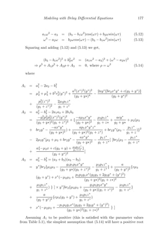
201. 146 Mathematical Modeling: Models, Analysis and Applications
Solution: The characteristic base curves for this initial value problem are
solutions of
dx
dt
= et
, x(0) = x0
x(t) = x0 + et
− 1
and along these curves
dρ(x(t), t)
dt
= 2ρ(x(t), t)
Solving, we get
ρ(x(t), t) = ρ(x(0), 0)e2t
= ρ(x0)e2t
ρ(x(t), t) = (1 + sin2
x0)e2t
,
after substituting the initial value for ρ0(x). Replacing x0 by x − et
+ 1, we
get the traffic density as
⇒ ρ(x, t) = [1 + sin2
(x − et
+ 1)]e2t
Problem 4.5.7 A reaction diffusion model is given by
∂M1
∂t
= r(a − M1 + M2
1 M2) +
∂2
M1
∂x2
∂M2
∂t
= r(b − M2
1 M2) + D
∂2
M2
∂x2
where M1 and M2 are morphogen concentrations. All the parameters
r, a, b, c, D are positive constants.
(i) Explain the model and find the non-zero homogenous steady state.
(ii) Show that the condition stability (without diffusion) is b−a−(a+b)3
0.
(iii) Linearize the system about the non-zero steady state and find the condi-
tion for diffusive instability.
Solution: A spatially homogeneous steady state (m∗
1, m∗
2) of the model is
given by
a − m∗
1 + (m∗
1)2
m∗
2 = 0
b − (m∗
1)2
m∗
2 = 0
Solving we get, (m∗
1, m∗
2) =
a + b,
b
(a + b)2
Let
M1(x, t) = m1(x, t) − m∗
1 (4.40)
M2(x, t) = m2(x, t) − m∗
2 (4.41)

202. Spatial Models Using Partial Differential Equations 147
be small non-homogeneous perturbations of the uniform steady state. Substi-
tuting (4.40) and (4.41) in the given system and retaining the linearized term
we get,
∂m1
∂t
= a11m1 + a12m2 +
∂2
m1
∂x2
(4.42)
∂m2
∂t
= a21m1 + a22m2 + D
∂2
m2
∂x2
(4.43)
where
a11 = (
∂f1
∂M1
)(m∗
1 ,m∗
2) =
b − a
b + a
; a12 = (
∂f1
∂M2
)(m∗
1 ,m∗
2) = (a + b)2
;
a21 = (
∂f2
∂M1
)(m∗
1 ,m∗
2 ) =
−2b
a + b
; a22 = (
∂f2
∂M2
)(m∗
1 ,m∗
2 ) = −(a + b)2
.
Let m1 = A1eλt
cos(qx) and m2 = A2eλt
cos(qx) be the solution of (4.42)
and (4.43). Then we get
A1
λ −
b − a
b + a
+ q2
) − A2(a + b)2
= 0
A1
2b
a + b
+ A2
λ + (a + b)2
+ Dq2
= 0
For a non-trivial solution of A1 and A2, we must have

208. λ − b−a
b+a + q2
(a + b)2
2b
a+b λ + (a + b)2
+ Dq2

214. = 0
⇒ λ2
−
b − a
b + a
− (a + b)2
− q2
(1 + D)
λ
+
b − a
b + a
− q2
−(a + b)2
− Dq2
+ 2b(a + b) = 0 (4.44)
Without diffusion, (4.44) reduces to
(λ)2
−
b − a
b + a
− (a + b)2
λ + (a + b)2
= 0 (4.45)
Therefore, the system will be stable (without diffusion) if
b − a
b + a
− (a + b)2
0
(b − a) − (a + b)3
0. (4.46)

215. 148 Mathematical Modeling: Models, Analysis and Applications
With diffusion, the system will be stable if
b − a
b + a
− (a + b)2
− q2
(1 + D) 0 (4.47)
(q2
−
b − a
b + a
)(Dq2
+ (a + b)2
) + 2b(a + b) 0 (4.48)
Clearly, (4.47) is always negative by virtue of (4.46). Therefore, the question
of diffusive instability will occur if (4.48) is violated, that is
(q2
−
(b − a)
(b + a)
)(Dq2
+ (a + b)2
) + 2b(b + a) 0
Dq4
+ {(a + b)2
− D
(b − a)
(b + a)
}q2
+ (a + b)2
0,
which is the required condition for diffusive instability.
4.6 Exercises
1. (i) Show that in polar coordinates defined by the relations x = rcosθ, y =
rsinθ, the Laplace equation ∇2
u = 0 takes the form
∂2
u
∂r2
+
1
r
∂u
∂r
+
1
r2
∂2
u
∂θ2
= 0
(ii) Consider a semicircular plate of radius a, which is insulated on both
faces. Its curved boundary is kept at constant temperature T0 and its
bounding diameter is kept at zero temperature. Write an appropriate
model using partial differential equations, stating the boundary condi-
tions clearly. Hence, obtain an expression for the steady state tempera-
ture distribution.
2. Let u(x, t) denote the temperature function in a rod of length L at any
point x at any time t. The sides of the rod are insulated and kept ini-
tially at temperature sin
πx
L
. The two ends of the rod are then quickly
insulated such that the temperature gradient is zero at each end.
(i) Formulate a mathematical model of the given situation using partial
differential equations, stating clearly the boundary and initial condi-
tions.
(ii) Using the method of separation of variables, obtain an expression
for the temperature u(x, t).
3. Let u(x, t) denote the temperature function in a rod of length L at any
point x at time t. The sides of the rod are insulated and kept initially at

216. Spatial Models Using Partial Differential Equations 149
temperature sin
nx
L
. Both ends of the rod are quickly cooled at 0 ◦
C
and are kept at that temperature.
(i) Formulate a mathematical model of the given situation using partial
differential equations, stating clearly the boundary and initial condi-
tions.
(ii) Using the method of separation of variables, obtain an expression
for the temperature u(x, t).
(iii) If the rod is initially kept at temperature x and u(x, t) → 0 for large
t(t → ∞), formulate a new mathematical model for u(x, t) and solve it.
(Assume that both ends of the rod are quickly cooled at 0o
C and are
kept at that temperature).
4. A homogenous flexible string is stretched between two fixed points, (0, 0)
and (l, 0). The string is released from rest from a position u(x, 0) =
μx(l − x). Through appropriate modeling, obtain an expression for the
displacement u(x, t) of the string at any time t.
5. The faces of a thin square plate of area π2
are perfectly insulated and
its four slides are kept at temperature zero. The initial temperature of
the plate is given by u(x, y, 0) = xy(π − x)(π − y), where u(x, y, t) gives
the temperature function of the square plate.
(i) Formulate a mathematical model of the given situation using partial
differential equations stating clearly the boundary and initial conditions.
(ii) Use the method of separation of variables to obtain an expression
for the temperature u(x, y, t) in the plate.
6. A homogenous flexible string of length L is stretched between (0, 0) and
(L, 0) and is released with a velocity ksin3
πx
L
parallel to the axis of
y from the equilibrium position. Let u(x, t) be the displacement of the
string at any time t.
(i) Formulate a mathematical model of the given situation using partial
differential equations, stating clearly the boundary and initial condi-
tions.
(ii) Using the method of separation of variables, obtain an expression
for the displacement u(x, t).
7. Find the traffic density ρ(x, t) satisfying
∂ρ
∂t
+
∂(ρu)
∂x
= 0,
where u, the velocity of the car, is a function of traffic density alone and
is given by
u(ρ) = umax
1 −
ρ
ρmax
2
, 0 ≤ ρ ρmax

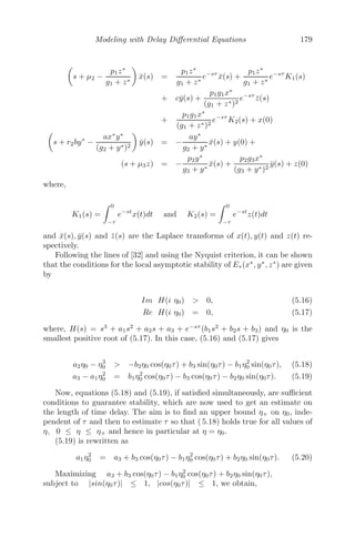
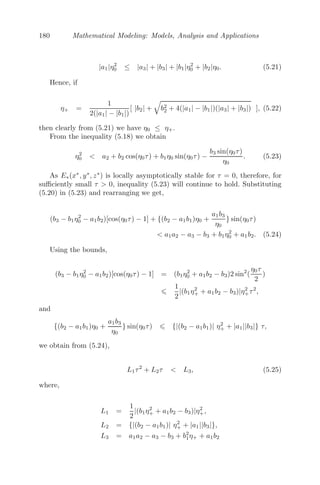
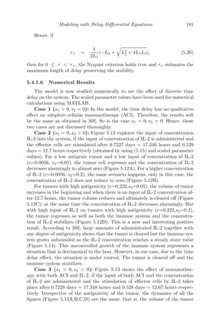
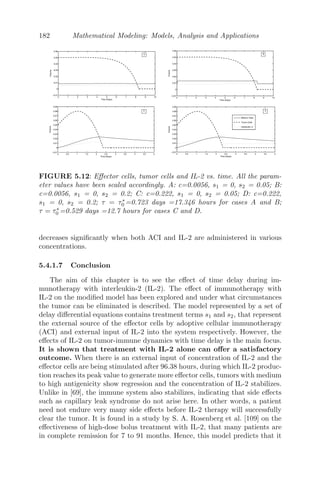
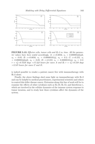
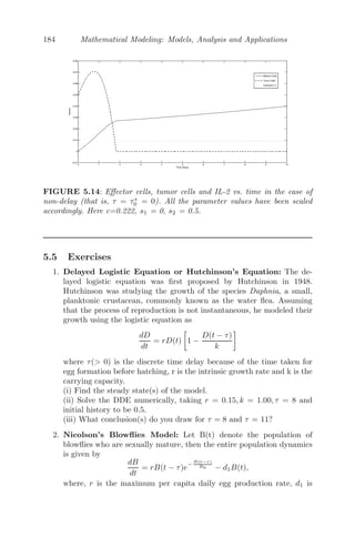
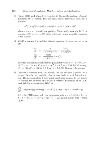
217. 150 Mathematical Modeling: Models, Analysis and Applications
with initial traffic density as
ρ(x, 0) =
⎧
⎨
⎩
150, x 0
150
1 − x
2
, 0 x 1
80, x 1
8. Find the traffic density ρ(x, t) satisfying the traffic equation
∂ρ
∂t
+ (1 − 2ρ)
∂ρ
∂x
= 0
with initial traffic density as
ρ(x, 0) =
⎧
⎨
⎩
1
4 , x 0
1
4 (1 − x2
)2
, x 1
0, x ≥ 1
9. Find the traffic density ρ(x, t) satisfying
(i)
∂ρ
∂t
+ 2
∂ρ
∂x
= 0, ρ0(x) = e−x2
(ii)
∂ρ
∂t
+ 2t
∂ρ
∂x
= 0, ρ0(x) = e−x2
(iii)
∂ρ
∂t
+ 2(1 − ρ)
∂ρ
∂x
= 0,
ρ0(x) =
1, x ≤ 0
0, x 0
10. The linear growth of a population is given by [26]
∂P(x, t)
∂t
= αP(x, t) + D
∂2
P(x, t)
∂x2
(i) Obtain the solution of the given model.
(ii) Let P(x, t) = k (constant). Then show that the value x
t is given by
x
t
= ∓
4αD −
2D
t
ln(t) −
2D
t
ln
√
2πD
k
P0
1/2
11. The spread of the spruce budworm [77] is given by
∂B
∂t
= αB
1 −
B
k
− β
B2
h2 + B2
+ D
∂2
B
∂x2
(i) Explain the model and find homogenous stability steady state(s).
(ii) Perform the linear stability analysis about the equilibrium point(s)
for the non-diffusive system and obtain the condition for stability. In-
terpret the condition in the context of the model.
(iii) Now, perform the linear stability analysis for a diffusive system and
conclude about the effect of diffusion on the system.

218. Spatial Models Using Partial Differential Equations 151
12. Segal and Jackson [119, 26] have modeled a spatially distributed
predator-prey system as
Prey :
∂V
∂t
= (k0 + k1V ) − AV E + μ2∇2
V
Predator :
∂E
∂t
= BV E − ME − CE2
+ μ2∇2
E
(i) Describe the model by explaining each term in the equations.
(ii) Assuming M = 0 and putting v = V B
k0
and e = Ec
k0
, write the model
in non-dimensionlized form as
∂v
∂t
= (1 + kv)v − aev + δ2
∇2
v
∂e
∂t
= ev − e2
+ ∇2
e
where k = k1
B , a = A
C and δ2
= μ1
μ2
.
(iii) Find the non-trivial homogenous steady state(s).
(iv) Show that the condition for diffusive instability is k−δ2
2
√
a − k.
13. The spread of least colonies was introduced by Gray and Kirwan [26, 48]
and is given by
∂Y
∂t
= D1
∂2
Y
∂x2
+ kY (G − G0)
∂G
∂t
= D2
∂2
G
∂x2
− ckY (G − G0)
Here, Y (x, t) is the density of yeast cells and G(x, t) is the glucose con-
centration in medium at time t and location x.
(i) Explain the model and find the homogenous steady state(s).
(ii) Perform the linear stability analysis about the equilibrium point(s)
for the non-diffusive system and obtain the condition for stability. In-
terpret the condition in context with the model.
(iii) Now, perform the linear stability analysis for the diffusive system
and comment about the effect of diffusion on the system.
14. A space dependent arms race model is given by [64]
∂A1(x, t)
∂t
= aA2
2 − mA1 + r + D1
∂2
A1
∂x2
∂A2(x, t)
∂t
= bA2
1 − nA2 + s + D2
∂2
A2
∂x2
where A1 and A2 are the amounts spent on arms by two countries C1
and C2, where the parameters a, b, m, n are positive.
(i) Explain the model and find the non-trivial homogenous steady

219. 152 Mathematical Modeling: Models, Analysis and Applications
state(s).
(ii) Using the Dirichlet boundary condition solve the model numerically
by taking appropriate values of a, b, m, n, r, s and comment on the re-
sult.
(iii) How does the result change if Neumann’s boundary condition is
used?
15. The model of reaction diffusion system is given by
∂M1
∂t
= αM1M2 − βM2
1 + δ2 ∂2
M1
∂x2
∂M2
∂t
= M2 − M1M2 + M2
2 +
∂2
M1
∂x2
where M1 and M2 are morphogen concentrations. All the parameters
α, β, δ are positive constants.
(i) Explain the model and find the non-zero equilibrium point (s).
(ii) Obtain the conditions for Turing instability and evaluate the values
of δ for which Turing instability can take place.

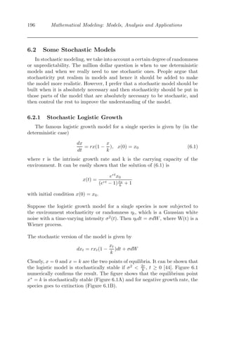
220. Chapter 5
Modeling with Delay Differential
Equations
5.1 Introduction ............................................................... 153
5.2 Different Models Using Delay Differential Equations ..................... 154
5.2.1 Delayed Protein Degradation ..................................... 154
5.2.2 Football Team Performance Model ............................... 155
5.2.3 Breathing Model .................................................. 156
5.2.4 Housefly Model .................................................... 157
5.2.5 Shower Problem ................................................... 158
5.2.6 Two-Neuron System ............................................... 159
5.3 Linear Stability Analysis .................................................. 160
5.3.1 Linear Stability Criteria ........................................... 161
5.4 Miscellaneous Examples ................................................... 163
5.4.1 A Research Problem: Immunotherapy with Interleukin-2, a Study
Based on Mathematical Modeling [8] ..................................... 171
5.4.1.1 Background of the Problem ............................. 171
5.4.1.2 The Model ............................................... 173
5.4.1.3 Positivity of the Solution ................................ 175
5.4.1.4 Linear Stability Analysis with Delay .................... 175
5.4.1.5 Estimation of the Length of Delay to Preserve Stability 178
5.4.1.6 Numerical Results ....................................... 181
5.4.1.7 Conclusion ............................................... 182
5.5 Exercises .................................................................. 184
5.1 Introduction
What are Delay Differential Equations (DDE)? is the first question that
comes to mind, when you begin reading this chapter. In layman’s terms, a
DDE is a differential equation in which the derivatives of some unknown func-
tions at present time are dependent on the values of the functions at previous
times. Let us consider a general DDE of the form
dx(t)
dt
= f(t, x(t), x(t − τ))
where x(t − τ) = {x(τ) : τ ≤ t} gives the trajectory of the solution in the
past. Here, the function f is a functional operator from ×n
×C1
to n
and
x(t)∈ n
. We will not provide a detailed discussion on DDEs that fall into
the class of functional differential equations. Interested readers are advised to
consult references [45, 71, 78].
153

221. 154 Mathematical Modeling: Models, Analysis and Applications
Now, what about the solutions of DDEs? It is not easy to solve a DDE
analytically. To give an idea of the process, let us consider a simple DDE of
the form
dx
dt
= −x(t − τ), t 0
Initial history: x(t)=1, −τ ≤ t ≤ 0. Clearly, with τ = 0, x(t) = x(0)e−t
.
However, the presence of τ makes the situation a bit tricky. Hence, in the
interval 0 ≤ t ≤ τ, we have
dx
dt
= −x(t − τ) = −1
⇒ x(t) = x(0) +
t
0
(−1)ds = 1 − t, 0 ≤ t ≤ τ.
In τ ≤ t ≤ 2τ, we get, 0 ≤ t − τ ≤ τ and so we have,
x(t) = −x(t − τ) = −[1 − (t − τ)]
⇒ x(t) = x(τ) +
t
τ
[−{1 − (s − τ)}]ds
x(t) = 1 − t +
(t − τ)2
2
, τ ≤ t ≤ 2τ
and so on. In general, it can be shown (use mathematical induction) that
x(t) = 1 +
n
k=1
(−1)k [t − k − 1 τ]k
k!
, (n − 1)τ ≤ t ≤ nτ, n ≥ 1
The above method is known as a procedure of steps. One can use MATLAB
DDE 23 to obtain numerical solutions of the DDEs.
5.2 Different Models Using Delay Differential Equations
5.2.1 Delayed Protein Degradation
Let P(t) be the concentration of proteins at any time t in a system, then
the production of proteins at any time is given by [12]
dP(t)
dt
= α − βP(t) − γP(t − τ),

222. Modeling with Delay Differential Equations 155
where α is the constant rate of protein production, β is the rate of non-
delayed protein degradation and γ is the rate of delayed protein degradation.
The discrete time delay τ is due to the fact that the protein degradation
machine degrades the protein after a time τ after initiation. Figure 5.1 shows
the degradation of protein for various parameter values, obtained from [12].
0 50 100 150 200
80
90
100
110
120
130
140
150
Time
Protein
Concentration
P(t)
0 50 100 150 200
20
30
40
50
60
70
80
Time
A B
FIGURE 5.1: The delay induced protein degradation. Part A shows a protein
delay with parameter values α = 40, β = 0.3, γ = 0.1, τ = 20 and initial
history 150. Part B shows an oscillatory behavior of protein degradation with
parameter values α = 100, β = 1.1, γ = 1, τ = 10 and initial history 20.
5.2.2 Football Team Performance Model
R.B. Banks [9] proposed a delay-induced mathematical model to analyze
the performance of a National Football League (NFL) football team during
the last 40 years. The proposed model is
dU
dt
= b
1
2
− U(t − z)
where U(t) is the fraction of games won by an NFL team during one season
and it lies between 0 and 1, and b is the growth rate. The computational
formula for U(t) is given by
U(t) =
1 × no. of games won + 1
2 × no. of games tied + 0 × no. of games lost
Total no. of games

223. 156 Mathematical Modeling: Models, Analysis and Applications
Basically, the proposed model says that at the present time, the rate of change
of U is proportional to the difference between U = 1
2 (average values) and the
values of U at some previous time t − τ. Banks [9] concluded from his model
that the time delay τ plays an important role in the ups and downs of a
football team and it experiences a simple periodicity, which is evident from
Figure 5.2.
1960 1965 1970 1975 1980 1985 1990
0
0.1
0.2
0.3
0.4
0.5
0.6
0.7
t (years)
U(t)
FIGURE 5.2: The performance of an NFL team from 1960 to 1992, with pa-
rameter values b = 0.785, τ = 2 years and initial history 0.4. The performance
of the team shows a cyclic behavior, which matches with data [9].
5.2.3 Breathing Model
The arterial carbon dioxide level controls our rate of breathing. A mathe-
matical model was first developed by Mackey and Glass [42], where they as-
sumed that carbon dioxide is produced at a constant rate λ due to metabolic
activity and its removal from the bloodstream is proportional to both the
current carbon dioxide concentration and to ventilation. Ventilation, which is
the volume of gas exchanged by the lungs per unit of time, is controlled by
the carbon dioxide level in the blood. The process is complex and involves
detection of carbon dioxide levels by receptors in the brain stem. This car-
bon dioxide detection and its subsequent adjustment to ventilation is not an
instantaneous process; there is a time lag due to the fact that the blood trans-
port from the lungs to the heart and then back to the brain requires time [65].
Thus, if C is the concentration of the carbon dioxide, then the rate of change
of concentration of carbon dioxide due to breathing is given by
dC(t)
dt
= λ − αVmaxC(t)V̇ (t − τ)
where V̇ (t) is the rate of ventilation and is assumed to follow the Hill function,
that is V̇ (t) = (C(t))n
θn+(C(t))n ; Vmax, θ, n and α are constants. Thus, the rate of

224. Modeling with Delay Differential Equations 157
change of concentration of carbon dioxide is given by
dC(t)
dt
= λ − αVmaxC(t)
(C(t − τ))n
θn + (C(t − τ))n
Figure 5.3 shows the oscillatory solution of the Mackey-Glass equation, rep-
resenting the carbon dioxide content.
0 0.5 1 1.5 2 2.5 3 3.5 4 4.5 5
0
0.2
0.4
0.6
0.8
1
1.2
1.4
1.6
1.8
Time
Carbondioxide
Content
C(t)
FIGURE 5.3: The oscillatory behavior of carbon dioxide content. The pa-
rameter values, obtained from [65], are λ = 6, α = 0.3, Vm = 0.1, θ = 1, n = 3,
initial history 1.2 and τ = 0.25.
5.2.4 Housefly Model
Taylor and Sokal [128] proposed a model to describe the behavior of the
adult housefly Musca domestic in laboratory conditions. To capture the dy-
namics of the housefly, the model is represented using a delay differential
equation as
dH
dt
= −d1H(t) + βH(t − τ)[k − βMH(t − τ)]
Here, H(t) represents the number of adult houseflies at any time t, d1 is the
natural death, τ(0) is the discrete time delay, which is the time from laying
eggs until their emerging from the pupal case (oviposition and eclosion of
adults), β is the number of eggs laid per adult, and assuming the number of
eggs laid is proportional to the number of adults, the number of new eggs
at time t − τ would be βH(t − τ). The term k − βMH(t − τ) gives the
egg-to-adult survival rate, k and M being the maximum egg-adult survival
rate and reduction in survival for each egg respectively. Figure 5.4 shows
periodic solution as observed in the behavior of adult houseflies in laboratory

225. 158 Mathematical Modeling: Models, Analysis and Applications
conditions [128]. Please note that for τ = 0, the housefly population follows a
logistic growth.
0 50 100 150 200 250 300
0
200
400
600
800
1000
1200
1400
t−Time
Number
of
Adult
Houseflies
H(t)
τ = 5
τ = 0
FIGURE 5.4: The oscillatory behavior of the adult houseflies. The parameter
values, obtained from [114, 128] are d1 = 0.147, β = 1.81, k = 0.5107, M =
0.000226, initial history 100 and τ = 5. The system follows a logistic growth
for τ = 0.
5.2.5 Shower Problem
People enjoy showering, especially when they are able to control the water
temperature. The dynamics of human behavior while taking a shower when
the water temperature is not comfortable, is quite interesting. A simple DDE
model is proposed to capture such dynamics. We assume that the speed of
water is constant (uniform flow) from the faucet to shower head, which takes
the time τ seconds (say). Let T (t) denote the temperature of water at the
faucet at time t, then the temperature evolution is given by
dT
dt
= −α[T (t − τ) − Td]
where Td is the desired temperature and α gives the measure of a person’s
reaction due to wrong water temperature. One type of person might prefer a
low value of α whereas another type of person would choose a higher value of α.
For α = 0.5, the temperature of the water goes to 40 ◦
C, which is comfortable
to the body and the person remains calm (Figure 5.5A). For α = 0.8 and 1.1,
after initial fluctuation, the temperature of the water goes to 40 ◦
C. A person

226. Modeling with Delay Differential Equations 159
0 5 10 15
0
5
10
15
20
25
30
35
40
45
Temperature
of
the
water
T(t)
0 5 10 15
0
10
20
30
40
50
60
0 5 10 15
0
10
20
30
40
50
60
70
0 5 10 15
−10
0
10
20
30
40
50
60
70
80
0 5 10 15
−200
−150
−100
−50
0
50
100
150
200
t−Time
0 5 10 15
−1.5
−1
−0.5
0
0.5
1
1.5
2
2.5
x 10
4 F
E
D
C
B
A
α = 0.5
α = 0.8 α = 1.1
α = 1.55 α = 1.8 α = 2.8
FIGURE 5.5: Varied temperatures of water for different values of α. The
parameter values are Td = 40 ◦
C, τ = 1, initial history = 0.5 and α =
0.5, 0.8, 1.1, 1.55, 1.8 and 2.8 respectively.
may show initial discomfort with the start of the shower (Figure 5.5B,C).
One person will prefer the value of α = 1.55 while showering (a bathroom
singer?), which shows cyclic behavior (Figure 5.5D). For α = 1.8 and 2.8,
the temperature of the water is erratic and unpleasant while taking shower
(Figure 5.5E,F).
5.2.6 Two-Neuron System
A two-neuron system of self-existing neurons is given by [7, 132]
du1
dt
= −u1(t) + a1tanh[u2(t − τ21)]
du2
dt
= −u2(t) + a2tanh[u1(t − τ12)]
where u1(t) and u2(t) are the activities of the first and second neurons re-
spectively, τ21 is the delay in signal transmission between the second neuron
and the first neuron (τ12 can be explained in similar manner) and ai’s (i
= 1,2) are the weighing of the connection between the neurons. By taking
a1 = 2, a2 = −1.5, τ12 = 0.2, τ21 = 0.5 such that τ12 + τ21 0.8, numerically
it has been shown that the model is asymptotically stable about the origin
(see Figure 5.6 A1,A2,A3). For τ12 = 0.4, τ21 = 0.6 such that τ12 + τ21 0.8,
a periodic solution bifurcates from the origin; that bifurcation is supercritical

227. 160 Mathematical Modeling: Models, Analysis and Applications
and the bifurcating periodic solution is orbitally asymptotically stable (see
Figure 5.6 B1,B2,B3). To learn more about the analytical calculations and
restrictions on τ12 and τ21, interested readers may go to [132], where it is
discussed in detail.
0 20 40 60 80 100
−0.3
−0.2
−0.1
0
0.1
0.2
0.3
0.4
t−Time
u
1
(t)
0 20 40 60 80 100
−0.4
−0.3
−0.2
−0.1
0
0.1
0.2
t−Time
u
2
(t)
−0.3 −0.2 −0.1 0 0.1 0.2 0.3 0.4
−0.4
−0.2
0
0.2
0.4
u
1
(t)
u
2
(t)
0 20 40 60 80 100
−0.5
0
0.5
t−Time
u
1
(t)
0 20 40 60 80 100
−0.5
0
0.5
t−Time
u
2
(t)
−0.5 0 0.5
−0.5
0
0.5
u 1
(t)
u
2
(t)
A1
A2
A3 B3
B2
B1
FIGURE 5.6: The activities of two self-exiting neurons. The parameter val-
ues, obtained from [114], are a1 = 2, a2 = −1.5 and initial history is (0.1,0.3).
Parts 5.6A1,A2,A3 show that the system is asymptotically stable about the ori-
gin for τ12 = 0.2, τ21 = 0.5 such that τ12 + τ21 0.8. For τ12 = 0.4, τ21 = 0.6
such that τ12 +τ21 0.8., Parts 5.6B1,B2,B3 illustrate that a periodic solution
bifurcates from the origin, which is orbitally asymptotically stable.
5.3 Linear Stability Analysis
We consider the delay differential equation
dx
dt
= −x(t − 1) (5.1)
and discuss its stability. Clearly, x = 0 is the only steady state solution. Since
the equation is linear, we try the exponential solution x = ceλt
, (c = 0) which

228. Modeling with Delay Differential Equations 161
gives
cλeλt
= −ceλ(t−1)
= −ceλt
e−λ
Let g(λ) ≡ λ + e−λ
= 0, (since ceλt
= 0)
This is the characteristics equation of 5.1, which is transcendental and has
infinitely many solutions. It is easy to check that the characteristics equation
λ + e−λ
= 0 has no real solution since g(λ) has an absolute minimum of 1 at
λ = 0. Therefore, we substitute λ = a + ib in the characteristics equation for
complex solutions and get
e−a−ib
+ a + ib = 0
⇒ e−a
(cos b − i sin b) + a + ib = 0
⇒ (e−a
cos b + a) + i(b − e−a
sin b) = 0
Equating the real and imaginary parts we get,
e−a
cos b = −a (5.2)
e−a
sin b = b (5.3)
Without any loss of generality, we assume b 0. We want to check whether
(5.2) and (5.3) can have solutions with positive values of real part a. Let us
assume that equations (5.2) and (5.3) have solutions with a 0. Then from
(5.2) we conclude that cos b 0, which implies b π
2 (since cos b 0 for
acute b). Now, for a 0, e−a
1 and | sin b| 1, implying |b| 1 (from 5.3).
This leads to a contradiction as b cannot simultaneously be greater than π
2
and numerically less than 1 in magnitude. Hence, we conclude that the real
part of the characteristic root cannot be positive, that is, it is negative and
hence the equilibrium point x = 0 is stable.
5.3.1 Linear Stability Criteria
The stability analysis in the previous section shows the complicated na-
ture of dealing with linear stability analysis of delay differential equations. In
this section, three theorems (without proofs) are stated, which may be used
directly to investigate linear stability analysis of delay differential equations.
Theorem 5.3.1.1 Consider a linear delay differential equation of the form
dx(t)
dt
= Ax(t) + Bx(t − τ)
where A, B are scalars whose equilibrium solution is x = 0, where A, B are
scalars. The corresponding characteristic equation is given by
λ = A + Be−λτ

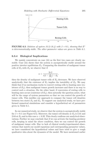
229. 162 Mathematical Modeling: Models, Analysis and Applications
Then [123],
(i) If A + B 0, then x = 0 is unstable.
(ii) If A + B 0 and B ≥ A, then x = 0 is asymptotically stable.
(iii) If A + B 0 and B A, then there exists τ∗
0 such that x = 0
is asymptotically stable for 0 τ τ∗
and unstable for τ τ∗
. Also, there
exists a pair of imaginary roots at τ = τ∗
= cos−1 −A/B
B2−A2 .
Theorem 5.3.1.2 Consider a linear autonomous delay differential equation
of the form
dx
dt
+ a1x(t − τ1) + a2x(t − τ2) = 0 (5.4)
where a1, a2, τ1, τ2 ∈ [0 , ∞). The transcendental characteristic equation of
(5.4) can be obtained by substituting the ansatz x(t) = ceλt
in (5.4), which
results in
λ + a1e−λτ1
+ a2e−λτ2
= 0 (5.5)
where λ is a complex number.
(i) Let a2 = 0 and a1, τ1 ∈ (0, ∞). A necessary and sufficient condition for
all roots of λ + a1e−λτ1
= 0 to have negative real parts is 0 a1τ1 π
2 .
(ii) Let a1, a2, τ1, τ2 ∈ (0, ∞). A sufficient condition for all roots of (5.5) to
have negative real parts is a1τ1 + a2τ2 1 and a necessary condition for the
same is a1τ1 + a2τ2 π/2.
Theorem 5.3.1.3 Consider the characteristic equation of the form
P(λ) + Q(λ)e−λτ
= 0
where P and Q are polynomials with real coefficients and τ( 0) is the discrete
time delay. Let,
(i) P(λ) = 0 in the region P(λ) ≥ 0,
(ii) Q(ib) |P(ib)|, 0 ≤ b ∞,
(iii) lim|λ|→∞, Re(λ)≥0 |Q(λ)
P (λ) | = 0, then, Real (λ) 0 for every root λ and all
τ ≥ 0.
Corollary: Suppose P(λ) has leading coefficient one and let Q(λ) = c
(constant). If
(i) all roots of the polynomial P(λ) are real and negative and |P(0)| |c| or
(ii) P(λ) = λ2
+ aλ + b, a, b 0 and either
(A1) b |c| and a2
≥ 2b or (A2) a
√
4b − a2 2|c| and a2
2b,
then Re(λ) 0 for every root λ and all τ ≥ 0.

230. Modeling with Delay Differential Equations 163
5.4 Miscellaneous Examples
Problem 5.4.1 Mackey-Glass Model: Mackey and Glass [42] proposed a
delayed model for the growth of density of blood cells
dB
dt
=
λαm
B(t − τ)
αm + Bm(t − τ)
− βB(t)
where λ, α, m, β and τ are positive constants.
(i) Explain the model in terms of the system parameters.
(ii) Solve the system numerically by taking λ = 0.2, α = 0.1, β = 0.1, m =
10, τ = 4 and initial history 0.1 and represent it graphically. What kind of
behavior is observed?
(iii) Obtain graphs by taking the discrete time delays τ = 6, 15, 30. What
changes do you observe in the dynamics of the system?
Solution: (i) B(t) is the density of blood cells in the circulating blood, λ
is the rate at which it is produced, α is the dissociation constant and β is the
rate of natural death of the cells. There is a release of mature cells from the
bone marrow into the blood due to the reduction in cells in the bloodstream
but there is a delay of approximately 6 days. Here, τ is the delay between
the production of blood cells in the bone marrow and its release into the
bloodstream. It is also assumed that the density of blood cells that enter the
bloodstream depends on cell density at an earlier time B(t − τ).
(ii) The numerical solution of the model shows that the density of blood
cells follows a damped oscillation for τ = 4 (see Figure 5.7A).
(iii) As the value of τ (=6) is increased, the system exhibits bifurcating
periodic solutions (Figure 5.7B). The solution becomes aperiodic for further
increase in τ = 15 (Figure 5.7C) and chaotic for τ = 30 (Figure 5.7D).
Problem 5.4.2 A second order delayed feedback system is given by [123]
d2
x
dt2
+
dx
dt
+ 3x = −
√
5 tanh[x(t − τ)]
Simulate the model numerically for τ = 0.5, 0.555, 0.6, 2, 3.5 and 5 and com-
ment on the dynamics of the system.
Solution: The second order delayed feedback system is first expressed as
a system of first order delayed differential equations
dx
dt
= y1
dy1
dt
= −y1 − 3x −
√
5 tanh[x(t − τ)]

231. 164 Mathematical Modeling: Models, Analysis and Applications
0 100 200 300 400 500
0
0.2
0.4
0.6
0.8
1
1.2
1.4
0 100 200 300 400 500
0
0.2
0.4
0.6
0.8
1
1.2
1.4
Density
of
Blood
Cells
B(t)
0 200 400 600 800 1000
0
0.2
0.4
0.6
0.8
1
1.2
1.4
0 200 400 600 800 1000
0
0.2
0.4
0.6
0.8
1
1.2
1.4
t−Time
A B
C D
FIGURE 5.7: The effect of delay on the density of blood cells with parameter
values λ = 0.2, α = 0.1, β = 0.1, m = 10 and initial history 0.1, obtained from
[114]. (A) This shows a damped oscillation for τ = 4. (B) As the value of delay
is increased to τ = 6, there is a cascading sequence of bifurcating periodic
solutions. (C) For further increase in delay, the solution becomes aperiodic
and (D) chaotic.
and then solved numerically for different values of τ. For τ = 0.5 and 3.5, the
system is asymptotically stable (see Figure 5.8A,E). For τ = 0.6 and 5, the
system is unstable (see Figure 5.8C,F). For τ = 0.555, the system bifurcates to
periodic solution (see Figure 5.8B) and for τ = 2.0, the system is in oscillatory
mode with high amplitude of oscillation (see Figure 5.8D).
Problem 5.4.3 Cooke proposed an epidemic model [75, 78] given by
dt
dt
= by(t − 7)[1 − y(t)] − cy(t),
where y(t) denotes the fraction of a population infected at time t.
(i) Find the equilibrium point(s) of the model and comment on their existence.
(ii) Investigate the stability of the system about the equilibrium point(s).
(iii) Simulate the model numerically for b = 2, c = 1, initial history = 0.8 and
comment on the dynamics of the system.

232. Modeling with Delay Differential Equations 165
0 20 40 60 80 100
−1.5
−1
−0.5
0
0.5
1
1.5
t−Time
x(t)
0 20 40 60 80 100
−0.1
−0.05
0
0.05
0.1
t−Time
x(t)
0 20 40 60 80 100
−0.015
−0.01
−0.005
0
0.005
0.01
0.015
t−Time
x(t)
0 20 40 60 80 100
−0.015
−0.01
−0.005
0
0.005
0.01
0.015
t−Time
x(t)
0 20 40 60 80 100
−1
−0.5
0
0.5
1
t−Time
x(t)
0 20 40 60 80 100
−0.2
−0.15
−0.1
−0.05
0
0.05
0.1
t−Time
x(t)
τ = 3.5
τ = 0.6
τ = 0.5
τ = 0.555
τ = 2.0
τ = 5.0
A
E
C
B
D
F
FIGURE 5.8: The effect of delay on the feedback system with initial history
(0.1,0.1). (A) Asymptotically stable, (B) periodic solution, (C) unstable, (D)
oscillatory mode with high amplitude, (E) asymptotically stable, (F) unstable.
Solution: (i) The equilibrium points are y∗
= 0 and y∗
= b−c
b . For the
existence of non-zero equilibrium points, we must have b c.
(ii) Putting y = Y + y∗
in the model equation and retaining the linear
terms only we get,
dt
dt
= b(1 − y∗
)y(t − 7) − (by∗
+ c)y(t).
For y∗
= 0,
dt
dt
= −cy(t) + by(t − 7).
Using Theorem 5.3.1.1, we get A+B = b−c 0 (or else non-zero equilibrium
points not exist). Hence, the system is unstable about the equilibrium point
y∗
= 0.
Note: One can also conclude if b c, the system is unstable and if b c, the
system is asymptotically stable about y∗
= 0. However, the system will have
only one positive equilibrium point in that case.
For y∗
= b−c
b ,
dt
dt
= −by(t) + cy(t − 7).

233. 166 Mathematical Modeling: Models, Analysis and Applications
Using Theorem 5.3.1.1, we get A + B = −(b − c) 0. The system is asymp-
totically stable about the equilibrium point y∗
= b−c
b if b c. However, if
b c, then there exists τ∗
0 such that x = 0 is asymptotically stable for
0 τ τ∗
and unstable for τ τ∗
.
(iii) Figure 5.9 shows the simulation of the model for b = 2, c = 1 and ini-
tial history = 0.8. The numerical solution agrees with the theory and the
graph shows that the system is stable and reaches the equilibrium solution
y∗
= b−c
b = 0.5 with time.
0 10 20 30 40 50 60 70 80
0.45
0.5
0.55
0.6
0.65
0.7
0.75
0.8
t−Time
Population
y(t)
FIGURE 5.9: The behavior of the population with time for b = 2, c = 1, τ = 7
and initial history 0.8.
Problem 5.4.4 Microbial Growth Model with Delay: A delayed bac-
terial growth model in a chemostat is given by (after scaling time and the
dependent variables) [28, 123]
dS(t)
dt
= 1 − S(t) −
mS(t)B(t)
a + S(t)
dB(t)
dt
= e−τ
m
S(t − τ)
a + S(t − τ)
B(t − τ) − B(t)
where S(t) is the substrate concentration (food for bacteria) and B(t) is the
biomass concentration of bacteria, m and a are positive constants and τ is the
time of cellular absorption resulting in the increase of bacterial biomass.
(i) Find the equilibrium point(s) of the model and comment on their existence.
(ii) Investigate the stability of the system about the equilibrium point(s).
(iii) Simulate the model numerically for m = 0.7, a = 2, τ = 0.1, initial history
= [2, 14] and comment on the dynamics of the system.

234. Modeling with Delay Differential Equations 167
Solution: (i) The equilibrium solutions (S∗
, B∗
) are obtained by solving
1 − S∗
−
mS∗
B∗
a + S∗
= 0
e−τ
m
S∗
a + S∗
B∗
− B∗
= 0,
where (S∗
, B∗
) are (i) (1,0), washout state and (ii)
aeτ
m−eτ , [1 − aeτ
m−eτ ]e−τ
,
survival state. The washout state always exists and the survival state exists if
e−τ m
1+a 1.
(ii) For linear stability analysis, the characteristic equation is obtained as

239. −1 + mB∗
S∗
(a+S∗)2 − mB∗
(a+S∗) − λ −mS∗
(a+S∗)
amB∗
e−τ
(a+S∗)2 e−λτ
−1 + mS∗
e−τ
a+S∗ e−λτ
− λ

244. = 0
For the washout state (1,0), the characteristic equation is given by

249. −1 − λ −m
(1+a)
0 −1 + me−τ
a+1 e−λτ
− λ

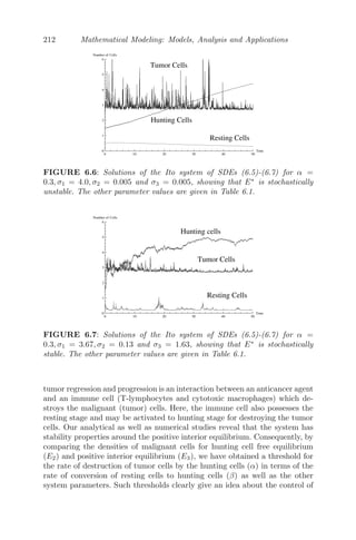
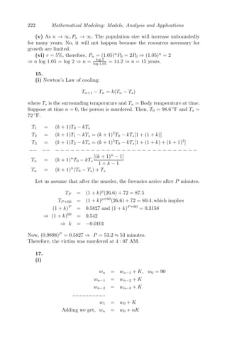
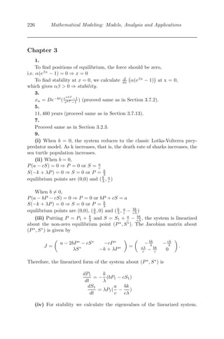
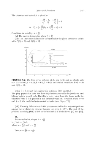
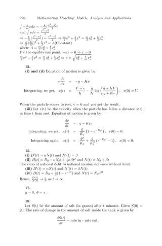
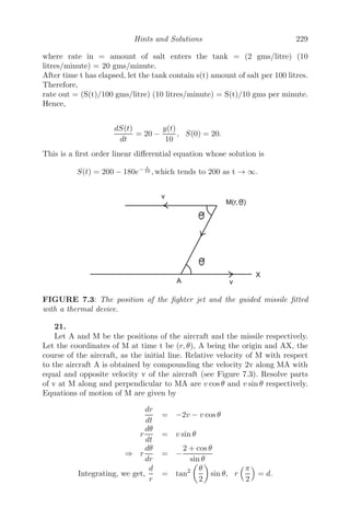
254. = 0
This is a transcendental equation, which has infinite many eigenvalues. One
of the eigenvalues is λ = −1. The rest are given by and λ = −1 + me−τ
a+1 e−τλ
.
Using Theorem 5.3.1.1, we get A = −1 and B = me−τ
a+1 . Clearly, B A and
A + B = −1 + me−τ
a+1 . Therefore, the washout state is stable if me−τ
a+1 1 and
unstable if me−τ
a+1 1 (please note that the survival state exists if the washout
state is unstable).
In a similar manner, for the survival state, the characteristic equation is
given by
(λ + 1)
λ + 1 −
me−τ
a + 1
e−τλ
= 0. (5.6)
Using Theorem 5.3.1.1, we conclude that the survival state (S∗
, B∗
) is always
asymptotically stable whenever it exists as A+B = −(1−S∗
)e−τ am
(a+S∗)2 0.
(iii) Numerical simulation is left to the reader (MATLAB code has been pro-
vided).
Problem 5.4.5 The delayed Lotka-Volterra competition system is given by
dx
dt
= x(t)[2 − αx(t) − βy(t − τ)]
dy
dt
= y(t)[2 − γx(t − τ) − δy(t)]
(i) Obtain the steady state solution(s).

255. 168 Mathematical Modeling: Models, Analysis and Applications
(ii) Investigate the stability of the non-zero steady state(s) for (a) α = δ = 2,
β = γ = 1; (b) α = δ = 1, β = γ = 2.
(iii) Simulate the model for (a) α = δ = 2, β = γ = 1; (b) α = δ = 1,
β = γ = 2 and comment on the dynamics of the system.
Solution: (i) The steady state solution(s) (x∗
, y∗
) are the solutions of
x∗
(2 − αx∗
− βy∗
) = 0
y∗
(2 − γx∗
− δy∗
) = 0,
which give the following: (0, 0);
2
α , 0
;
0, 2
δ
;
2(δ−β)
αδ−βγ , 2(α−γ)
αδ−βγ
. For linear sta-
bility analysis, the characteristic equation is given by

259. 2 − 2αx∗
− βy∗
− λ −βx∗
e−λτ
−γy∗
e−λτ
2 − γx∗
− 2δy∗
− λ

263. = 0
(iia) For α = δ = 2, β = γ = 1, the non-zero steady state solution is
2
3 , 2
3
and the corresponding characteristic equation is of the form
P(λ) + Q(λ)e−λτ
= 0,
where P(λ) =
λ +
4
3
λ +
4
3
and Q(λ) = −
4
3
.
Clearly, the leading coefficient of P(λ) is one and Q(λ) = −4
3 is a constant.
Moreover, all the roots of P(λ) are real and negative and |P(0)| = 16
3
|Q(λ)| = 4
3 . Therefore, by the corollary of Theorem 5.3.1.3, we conclude that
Re(λ) 0 for every root λ and all τ ≥ 0. Therefore, the given system is
asymptotically stable.
(iib) For α = δ = 1, β = γ = 2, the non-zero steady state solution is again
2
3 , 2
3
and the corresponding characteristic equation is of the form
P(λ) + Q(λ)e−λτ
= 0,
where P(λ) =
λ +
2
3
λ +
2
3
and Q(λ) = −
16
3
.
Clearly, the leading coefficient of P(λ) is one and Q(λ) = −16
3 is a con-
stant. Moreover, all the roots of P(λ) are real and negative but |P(0)| = 4
3 ≯
|Q(λ)| = 16
3 . Therefore, one of the criteria of the corollary of Theorem 5.3.1.3
is violated and we conclude that the given system is unstable.
(iii) Numerical simulation is left to the reader (MATLAB code has been
given).
Problem 5.4.6 Delayed Gene Regulatory System: A negative feedback

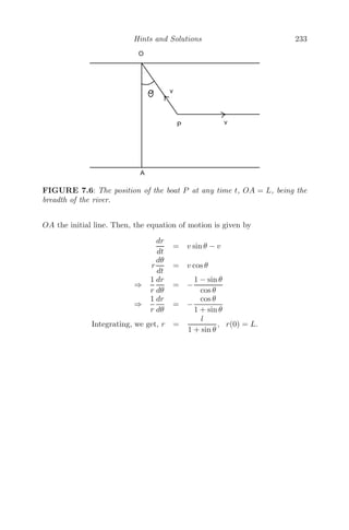
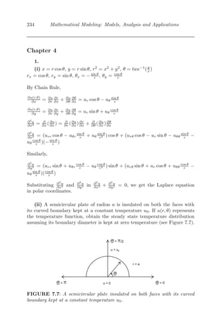
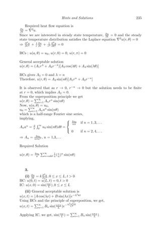
264. Modeling with Delay Differential Equations 169
gene regulatory system is described by a system of ODEs as [123]
dR(t)
dt
=
gm
1 +
P (t−τ)
k
n − α1R(t)
dP(t)
dt
= R(t) − α2P(t)
where, R(t) and P(t) represent the intracellular mRNA and the protein product
of the gene respectively. The growth of mRNA follows a Hill function, α1 and
α2 are the rates of degradation of mRNA and the protein product of the gene
respectively. The discrete time delay τ is the time taken by mRNA to leave
the nucleus, undergo protein synthesis in the ribosome, whereupon the protein
re-enters the nucleus and suppresses its own mRNA production.
(i) Solve the system numerically by taking gm = 1, k = 0.5, n = 3, α1 = α2 =
1, τ = 0.5 and represent it graphically.
(ii) By taking large values of the discrete time delay τ = 3.5, what changes do
you observe in the dynamics of the system?
Solution: (i) The model equation is solved numerically and the graphical
representation is shown in Figure 5.10A,B. Both the state variables R(t) and
P(t) converge to equilibrium solutions for τ = 0.5.
(ii) For large τ (= 3.5), we observe sustained oscillations as seen in Figure
5.10C,D.
Problem 5.4.7 Cargo pendulation reduction problem: Bridge cranes or
overload cranes are used in shipyards, railyards and warehouses to lift several
hundred tons of containers and move them to another place. Henry et al. [51]
and Masoud et al. [81] proposed a delay-induced mathematical model for safe
control of the crane pendulation as
d2
θ
dt2
+
dθ
dt
+ sinθ = −kcosθ[θ(t − τ) − θ]
where θ represents the angle due to pendulation. The aim is to stabilize the
system by reducing θ significantly at the end of the motion for safe operation.
(i) Show that for small θ and small τ, the system reduces to
d2
θ
dt2
+ ( − k τ)
dθ
dt
+ θ = 0
(ii) Solve numerically the system for τ = 12, = 0.1, k = −0.15, θ
(0) = 0
and θ(0) = 1 for −τ t 0 and comment on the result.
(iii) How do the dynamics change if θ
(0) = 0 and θ = 1.5 for −τ t 0?
Solution: (i) Clearly, θ = 0 is an equilibrium point. Near the steady state
solution θ = 0, sin(θ) ≈ θ, cos(θ) ≈ 1 and the model becomes
d2
θ
dt2
+
dθ
dt
+ θ = −k[θ(t − τ) − θ)]

265. 170 Mathematical Modeling: Models, Analysis and Applications
0 5 10 15 20
0.1
0.2
0.3
0.4
0.5
0.6
0.7
0.8
t−Time
Intercellular
mRNA
R(t)
0 5 10 15 20
0.1
0.2
0.3
0.4
0.5
0.6
t−Time
Protein
product
of
the
gene
P(t)
0 10 20 30 40 50
−0.5
0
0.5
1
1.5
2
t−Time
Intercellular
mRNA
R(t)
0 10 20 30 40 50
−0.2
0
0.2
0.4
0.6
0.8
1
1.2
1.4
t−Time
Protein
product
of
the
gene
P(t)
A B
C D
FIGURE 5.10: The numerical solution of the model equation with parameter
values gm = 1, k = 0.5, n = 3, α1 = α2 = 1, τ = 0.5 and initial history [0.1,
0.1]. (i) Figure 5.10A,B shows convergence to steady state solution for τ = 0.5
and (ii) Figure 5.10C,D shows sustained oscillations for τ = 3.5.
Now, for small τ, θ(t − τ) ≈ θ − τ θ
dt and the above equation reduces to
d2
θ
dt2
+
dθ
dt
+ θ = −k[θ − τ
θ
dt
− θ)]
⇒
d2
θ
dt2
+ ( − k τ)
dθ
dt
+ θ = 0
(ii) Graphical representation of the numerical solution for the given parame-
ters shows that the oscillations are damped (Figure 5.11A) for small amplitude
perturbation of the steady state solution θ = 0.
(iii) When the value of θ(0) is changed from 1.0 to 1.5, graphical represen-
tation of the numerical solution shows that the perturbation is large enough
to make the oscillation of the crane pendulation sustained (Figure 5.11B).

266. Modeling with Delay Differential Equations 171
0 50 100 150 200 250 300
−0.8
−0.6
−0.4
−0.2
0
0.2
0.4
0.6
0.8
1
t−Time
θ(t)
0 50 100 150 200 250 300
−2
−1.5
−1
−0.5
0
0.5
1
1.5
2
t−Time
θ(t)
A B
FIGURE 5.11: The numerical solution of the model equation with parameter
values = 0.1, k = −0.15 and initial history (i) θ
(0) = 0 and θ(0) = 1 (A),
(ii) θ
(0) = 0 and θ(0) = 1.5 (B).
5.4.1 A Research Problem: Immunotherapy with Interleukin-
2, a Study Based on Mathematical Modeling [8]
5.4.1.1 Background of the Problem
The mechanism of establishment and destruction of cancer, one of the
greatest killers in the world, is still a puzzle. Modern treatment involves
surgery, chemotherapy and radiotherapy, yet relapses occur. Hence, the need
for more successful treatment is clear. Developing schemes for immunotherapy
or its combination with other therapy methods are the major focus at present,
and aim at reducing the tumor mass, heightening tumor immunogenicity and
removal of immunosuppression induced in an organism in the process of tumor
growth. Recent progress has been achieved through immunotherapy, which
refers to the use of cytokines (protein hormones that mediate both natural
and specific immunities) usually together with adoptive cellular immunother-
apy (ACI) [37, 66, 108, 109, 118].
The main cytokine responsible for lymphocyte activation, growth and dif-
ferentiation is interleukin-2 (IL-2), which is mainly produced by T helper cells
(CD4+ T-cells) and in relatively small quantities by cytotoxic T-lymphocytes
(CD8+ T-cells). CD4 lymphocytes differentiate into T-Helper 1 and T-Helper
2 functional subjects due to the immune response. IL-2 acts in an autocrine
manner on T-Helper 1 and also induces the growth of T-Helper 2 and CD8
lymphocytes in a paracrine manner. The T-lymphocytes themselves are stim-
ulated by the tumor to induce further growth. Thus the complete biological
assumption of adoptive cellular immunotherapy is that the immune system
is expanded in number artificially (ex vivo) in cell cultures by means of hu-

267. 172 Mathematical Modeling: Models, Analysis and Applications
man recombinant interleukin-2. This can be done in two ways, either by (i)
lymphokine-activated killer cell therapy (LAK-therapy), where the cells are
obtained from the in vitro culturing of peripheral blood leukocytes removed
from patients with a high concentration of IL-2, or (ii) tumor-infiltrating lym-
phocyte therapy (TIL), where the cells are obtained from lymphocytes recov-
ered from the patient tumors, which are then incubated with high concentra-
tions of IL-2 in vitro and are comprised of activated natural killer (NK) cells
and cytotoxic T-lymphocyte (CTL) cells. The TIL are then returned into the
bloodstream, along with IL-2, where they can bind to and destroy the tu-
mor cells. It has been established clinically that immunotherapy with IL-2
has enhanced CTL activity at different stages of tumor [108, 109, 118]. Also,
there is evidence of the restoration of the defective NK cell activity as well
as enhancement of polyclonal expansion of CD4+ and CD8+ T cells [110, 127].
Kirschner and Panetta have studied the role of IL-2 in tumor dynamics,
particularly long-term tumor recurrence and short-term oscillations, in math-
ematical perspective [69]. The model proposed there deals with three popu-
lations; namely, the activated immune-system cells (commonly called effector
cells), such as cytotoxic T cells, macrophages and NK cells that are cytotoxic
to the tumor cells, the tumor cells and the concentration of IL-2. The impor-
tant parameters in their study are antigenicity of tumor (c), a treatment term
that represents external source of effector cells (s1) and a treatment term that
represents an external input of IL-2 into the system (s2). Their results can
be summarized as follows: (i) For non-treatment cases (s1 = 0, s2 = 0), the
immune system is not been able to clear the tumor for low-antigenic tumors,
while for highly antigenic tumors, reduction to a small dormant tumor is the
best-case scenario. (ii) The effect of adoptive cellular immunotherapy (ACI)
(s1 0, s2 = 0) alone can yield a tumor-free state for tumors of almost any
antigenicity, provided the treatment concentration is above a given critical
level. However, for tumors with small antigenicity, early treatment is needed
while the tumor is small, so that the tumor can be controlled. (iii) Treatment
with IL-2 alone (s1 = 0, s2 0) shows that if IL-2 administration is low, there
is no tumor-free state. However, if IL-2 input is high the tumor can be cleared
but the immune system grows without bounds, causing problems such as cap-
illary leak syndrome. (iv) Finally, the combined treatment with ACI and IL-2
(s1 0, s2 0) gives the combined effects obtained from the monotherapy
regime. For any antigenicity, there is a region of tumor clearance. These re-
sults indicate that treatment with ACI may be a better option either as a
monotherapy or in conjunction with IL-2. Here I have proposed a modifica-
tion of the model studied by Kirschner and Panetta by adding a discrete time
delay which exists when activated T-cells produce IL-2.

268. Modeling with Delay Differential Equations 173
5.4.1.2 The Model
The proposed model is an extension of the Kirschner-Panetta ordinary
differential equation model [69]
dE
dt1
= cT +
p1EIL
g1 + IL
− μ2E + s1
dT
dt1
= r2(1 − bT )T −
aET
g2 + T
dIL
dt1
=
p2ET
g3 + T
− μ3IL + s2
to a DDE model with proper biological justifications and is given by
dE
dt1
= cT +
p1E(t1 − τ)IL(t1 − τ)
g1 + IL(t1 − τ)
− μ2E + s1
dT
dt1
= r2(1 − bT )T −
aET
g2 + T
dIL
dt1
=
p2ET
g3 + T
− μ3IL + s2
Using the following scaling [69]
x = E
E0
, y = T
T0
, z = IL
IL0
, t = tst1; c̄ = cT0
tsE0
, ¯
p1 = p1
ts
,
¯
g1 = g1
IL0
, ¯
μ2 = μ2
ts
, ¯
g2 = g2
T0
, b̄ = bT0, , ¯
r2 = r2
ts
, ā = aE0
tsT0
,
¯
μ3 = μ3
ts
, ¯
p2 = p2E0
tsIL0
, ¯
g3 = g3
T0
, ¯
s1 = s1
tsE0
, ¯
s2 = s2
tsIL0
,
the given system is non-dimensionalized, given by (after dropping the overbar
notation for convenience)
dx
dt
= cy +
p1x(t − τ)z(t − τ)
g1 + z(t − τ)
− μ2x + s1
dy
dt
= r2(1 − by)y −
axy
g2 + y
(5.7)
dz
dt
=
p2xy
g3 + y
− μ3z + s2
subject to the following initial conditions
x(θ) = ψ1(θ), y(θ) = ψ2(θ), z(θ) = ψ3(θ)
ψ1(θ) ≥ 0, ψ2(θ) ≥ 0, ψ3(θ) ≥ 0; θ ∈ [−τ, 0] (5.8)
ψ1(0) 0, ψ2(0) 0, ψ3(0) 0;
where C+ = (ψ1(θ), ψ2(θ), ψ3(θ)) ∈ C([−τ, 0], R3
+0), the Banach space of con-
tinuous functions mapping the interval [−τ, 0] into R3
+0, where R3
+0 is defined
as
R3
+0 = ((x, y, z) : x, y, z ≥ 0) and R3
+, the interior of R3
+0 as
R3
+ = ((x, y, z) : x, y, z 0)

269. 174 Mathematical Modeling: Models, Analysis and Applications
In the system described by (5.7), x(t), y(t) and z(t) respectively represent
the effector cells, the tumor cells and the concentration of IL-2 in the single
site compartment. The first equation of the system (5.7) describes the rate of
change for the effector cell population. The effector cells grow due to the direct
presence of the tumor, given by the term cy, where c is the antigenicity of the
tumor. It is also stimulated by IL-2 that is produced by effector cells in an
autocrine and paracrine manner (the term p1xz
g1+z , where p1 is the rate at which
effector cells grow, and g1 is the half saturation constant). Clinical trials show
that there are immune stimulation effects from treatment with IL-2 [110, 127]
and there is a time lag between the production of IL-2 by activated T-cells and
the effector cell stimulation from treatment with IL-2. Hence, a discrete time
delay is being added to the second term of the first equation of the system
(5.7), which modifies to p1x(t−τ)z(t−τ)
g1+z(t−τ) , where μ2x gives the natural decay of
the effector cells and s1 is the treatment term that represents the external
source of the effector cells such as ACI. A similar type of term was introduced
by Galach [35] in his model equation, where he assumed that the source of the
effector cells is the term x(t − τ)y(t − τ), as the immune system needs some
time to develop a suitable response.
The second equation of the system (5.7) shows the rate of change of the
tumor cells, which follows logistic growth (a type of limiting growth). Due
to tumor-effector cell interaction, there is a loss of tumor cells at the rate a
and which is modeled by Michaelis Menten kinetics to indicate the limited
immune response to the tumor (the term axy
g2+y , where g2 is a half saturation
constant). The third equation of the system (5.7) gives the rate of change for
the concentration of IL-2. Its source is the effector cells that are stimulated by
interaction with the tumor and also has Michaelis Menten kinetics to account
for the self-limiting production of IL-2 (the term p2xy
g3+y , where p2 is the rate
of production of IL-2 and g3 is a half saturation constant), μ3z is the natural
decay of the IL-2 concentration and s2 is a treatment term that represents an
external input of IL-2 into the system.
Proper scaling is needed as the system is numerically stiff, and numerical
routines used to solve these equations will fail without scaling or inappropriate
scaling (in this case, a proper choice of scaling is E0 = T0 = IL0 = 1/b and
ts = r2 [69]). The parameter values have been obtained from [69], which is
put in tabular form (Table 5.1). The units of the parameters are in day−1
,
except of g1, g2, g3 and b, which are in volumes.
The aim of this problem is to study this modified model and to explore any
changes in the dynamics of the system that may occur when a discrete time
delay has been added in the system and to compare with the results obtained
by Kirschner and Panetta in [69].

270. Modeling with Delay Differential Equations 175
TABLE 5.1: Parameter Values Used for Numerical Simulation.
Parameters Values Scales Values
c (antigenicity of tumor) 0 ≤ c ≤ 0.05 0 ≤ c ≤ 0.278
p1 (growth rate of effector cells) 0.1245 0.69167
g1 (half saturation constant) 2 × 107
0.02
μ2 (natural decay rate of effector cells) 0.03 0.1667
r2 (growth rate of tumor cells) 0.18 1
b (1/carrying capacity of tumor cells) 1.0 × 10−9
1
a (decay rate of tumor) 1 5.5556
g2 (half saturation constant) 1 × 105
0.0001
μ3 (natural decay rate of IL-2) 10 55.556
p2 (growth rate of IL-2) 5 27.778
g3 (half saturation constant) 1 × 103
0.000001
5.4.1.3 Positivity of the Solution
The system of equations is now put in a vector form by setting
X = col(M, N, Z) ∈ R3
+0,
F(X) =
⎛
⎝
F1(X)
F2(X)
F3(X)
⎞
⎠ =
⎛
⎜
⎝
cy + p1x(t−τ)z(t−τ)
g1+z(t−τ) − μ2x + s1
r2(1 − by)y − axy
g2+y
p2xy
g3+y − μ3z + s2
⎞
⎟
⎠ ,
where F : C+ → R3
+0 and F ∈ C∞
(R3
+0). Then system (5.7) becomes
Ẋ = F(Xt), (5.9)
where · ≡ d/dt and with Xt(θ) = X(t + θ), θ ∈ [−τ, 0] [50]. It is easy to check
in equation (5.9) that whenever we choose X(θ) ∈ C+ such that Xi = 0, then
we obtain Fi(X)|Xi(t)=0,Xt∈C+
≥ 0, i = 1, 2, 3. Due to the lemma in [134], any
solution of equation (5.9) with X(θ) ∈ C+, say, X(t) = X(t, X(0)), is such
that X(t) ∈ R3
+0 for all t 0.
5.4.1.4 Linear Stability Analysis with Delay
The equilibria for the system (scaled) are as follows: (i) The x − z planar
equilibrium is ( s1(g1μ3+s2)
μ2(g1μ3+s2)−p1s2
, 0, s2
μ3
) and exists if μ2 p1s2
g1μ3+s2
.
(ii) The interior equilibrium is E∗(x∗
, y∗
, z∗
) where x∗
= r2
a (1 − by∗
)(g2 + y∗
),
z∗
= (p2r2(1−by∗
)(g2+y∗
)
aμ3(g3+y∗) + s2
μ3
) and y∗
is given by the equation cy∗
− μ2x∗
+
p1x∗
z∗
g1+z∗ + s1 = 0.
In the case of positive delay, the characteristic equation for the linearized
equation around the point (x∗
, y∗
, z∗
) is given by
P(λ) + Q(λ)e−λτ
= 0 (5.10)

271. 176 Mathematical Modeling: Models, Analysis and Applications
where
P(λ) = λ3
+ a1λ2
+ a2λ + a3
Q(λ) = b1λ2
+ b2λ + b3
a1 = μ2 + μ3 + br2y∗
−
ax∗
y∗
(g2 + y∗)2
a2 = br2y∗
(μ3 −
p1z∗
g1 + z∗
) +
ap1x∗
y∗
z∗
(g2 + y∗)2(g1 + z∗)
−
μ3p1z∗
g1 + z∗
+
acy∗
(g2 + y∗)
+ μ2{μ3 + br2y∗
−
ax∗
y∗
(g2 + y∗)2
}
a3 = bμ2μ3r2y∗
−
aμ2μ3x∗
y∗
(g2 + y∗)2
+
acμ3y∗
(g2 + y∗)
−
bg1p1p2r2x∗
(y∗
)2
(g3 + y∗)(g1 + z∗)2
+
ag1g3p1p2(x∗
)2
y∗
(g2 + y∗)(g3 + y∗)2(g1 + z∗)2
+
ag1p1p2(x∗
)2
(y∗
)2
(g2 + y∗)2(g3 + y∗)(g1 + z∗)2
+
aμ3p1x∗
y∗
z∗
(g2 + y∗)2(g1 + z∗)
−
bμ3p1r2y∗
z∗
g1 + z∗
+
bg1p1p2r2x∗
(y∗
)2
(g3 + y∗)(g1 + z∗)2
b1 = −
p1z∗
g1 + z∗
b2 = −
g1p1x∗
y∗
(g3 + y∗)(g1 + z∗)2
0
b3 =
ag1p1p2{g2g3 + 2g3y∗
+ (y∗)2
}x∗
y∗
(g2 + y∗)2(g3 + y∗)2(g1 + z∗)2
−
br2g1p1p2x∗
(y∗
)2
(g3 + y∗)(g1 + z∗)2
The steady state is stable in the absence of delay (τ = 0) if the roots of
P(λ) + Q(λ) = 0
⇒ λ3
+ (a1 + b1)λ2
+ (a2 + b2)λ + a3 + b3 = 0 (5.11)
have negative real parts. This occurs if and only if a1 +b1 0, a3 +b3 0 and
(a1 + b1)(a2 + b2) − (a3 + b3) 0 (by Routh Hurwitz’s criteria). This implies
μ2 + μ3 + br2y∗
−
ax∗
y∗
(g2 + y∗)2
−
p1z∗
g1 + z∗
0
p1
g1p2x∗
y∗
μ3(g3 + y∗)(g1 + z∗)2
+
z∗
g1 + z∗
μ2 p1{
z∗
g1 + z∗
+
g1p2x∗
(g2g3 + 2g3y∗
+ (y∗)2
)
μ3(g3 + y∗)2(g1 + z∗)2
}
(The above criteria is satisfied with the set of parameters shown in Section
5.4.1.2, provided 0 ≤ c ≤ 0.278, s2 μ2μ3g1
p1−μ2
). Now substituting λ = iω (where
ω is positive) in equation (5.10) and separating the real and imaginary parts
we obtain the system of transcendental equations

272. Modeling with Delay Differential Equations 177
a1ω2
− a3 = (b3 − b1ω2
)cos(ωτ) + b2ωsin(ωτ) (5.12)
ω3
− a2ω = b2ωcos(ωτ) − (b3 − b1ω2
)sin(ωτ) (5.13)
Squaring and adding (5.12) and (5.13) we get,
(b3 − b1ω2
)2
+ b2
2ω2
= (a1ω2
− a3)2
+ (ω3
− a2ω)2
⇒ ρ3
+ A1ρ2
+ A2ρ + A3 = 0, where ρ = ω2
(5.14)
where
A1 = a2
1 − 2a2 − b2
1
= μ2
2 + μ2
3 + b2
r2
2(y∗
)2
+
a2
(x∗
)2
(y∗
)2
(g2 + y∗)4
−
2ay∗
{br2x∗
y∗
+ c(g2 + y∗
)}
(g2 + y∗)2
+
p2
1(z∗
)2
(g1 + z∗)2
−
2μ2p1z∗
g1 + z∗
A2 = a2
2 − b2
2 − 2a1a3 + 2b1b3
=
−g2
1p2
1p2
2(x∗
)2
(y∗
)2
(g3 + y∗)2(g1 + z∗)4
+ {
−aμ3x∗
y∗
(g2 + y∗)2
−
μ3p1z∗
g1 + z∗
+
acy∗
g2 + y∗
+ μ2(μ3
+ br2y∗
−
−ax∗
y∗
(g2 + y∗)2
) +
ap1x∗
y∗
z∗
(g2 + y∗)2(g1 + z∗)
+ br2y∗
(μ3 −
p1z∗
g1 + z
)}2
− 2μ3y∗
[μ2 + μ3 + br2y∗
−
ax∗
y∗
(g2 + y∗)2
−
p1z∗
g1 + z∗
] [br2(μ2 −
p1z∗
g1 + z∗
+
a{−μ2x + c(g2 + y) + μ3p1z∗
g1+z∗ }
(g2 + y∗)2
]
A3 = a2
3 − b2
3 = (a3 + b3)(a3 − b3)
= y∗
[br2{μ2μ3 −
g1p1p2x∗
y∗
(g3 + y∗)(g1 + z∗)2
−
μ3p1z∗
g1 + z∗
} +
a
(g2 + y∗)2
{cμ3
(g2 + y∗
) + x∗
(−μ2μ3 +
p1p2g1x∗
(g2g3 + 2g3y∗
+ (y∗
)2
)
(g3 + y∗)2(g1 + z∗)2
+
μ3p1z∗
g1 + z∗
) } ] × y∗
[br2{μ2μ3 +
g1p1p2x∗
y∗
(g3 + y∗)(g1 + z∗)2
−
μ3p1z∗
g1 + z∗
}
+
a
(g2 + y∗)2
{cμ3(g2 + y∗
) +
μ3p1z∗
g1 + z∗
)
+ x∗
(−μ2μ3 +
−p1p2g1x∗
(g2g3 + 2g3y∗
+ (y∗
)2
)
(g3 + y∗)2(g1 + z∗)2
} ]
Assuming A1 to be positive (this is satisfied with the parameter values
from Table 5.1), the simplest assumption that (5.14) will have a positive root

273. 178 Mathematical Modeling: Models, Analysis and Applications
is A3 = a2
3 − b2
3 0. Since (a3 + b3) is positive (from the non-delay case), we
must have (a3 − b3) 0 and this gives
y∗
[br2{μ2μ3 +
p1(g1p2x∗
y∗
g3+y∗ − μ3z∗
(g1 + z∗
))
(g1 + z∗)2
}br2y∗
−
ax∗
y∗
(g2 + y∗)2
−
p1z∗
g1 + z∗
0
p1{
g1p2x∗
y∗
μ3(g3 + y∗)(g1 + z∗)2
+
z∗
g1 + z∗
} μ2
p1{
g1p2x∗
(g2g3 + 2g3y∗
+ (y∗)2
)
μ3(g3 + y∗)2(g1 + z∗)2
+
z∗
g1 + z∗
}
Hence, we can say that there is a positive ω0 satisfying (5.14), that is, the
characteristic equation (5.10) has a pair of purely imaginary roots of the form
± iω0. Eliminating sin(τω) from (5.12) and (5.13), we get,
cos(ωτ) =
(a1ω2
− a3)(b3) + (ω3
− a2ω)(b2ω)
(b3)2 + (b2ω)2
Then τ∗
n corresponding to ω0 is given by
τ∗
n =
1
ω0
arccos[
(a1ω2
0 − a3)(b3) + (ω3
0 − a2ω0)(b2ω0)
(b3)2 + (b2ω0)2
] +
2nπ
ω0
(5.15)
For τ = 0, E∗ is stable. Hence, E∗ will remain stable for τ τ0 where
τ0 = τ∗
0 as n = 0 [33].
5.4.1.5 Estimation of the Length of Delay to Preserve Stability
The linearized form of the system (5.7) is
dx
dt
=
p1z∗
g1 + z∗
− μ2
x +
p1z∗
g1 + z∗
x(t − τ) + cy +
p1g1x∗
(g1 + z∗)2
z(t − τ)
dy
dt
= −
ay∗
g2 + y∗
x +
ax∗
y∗
(g2 + y∗)2
− r2by∗
y
dz
dt
= −
p2y∗
g3 + y∗
x +
p2g3x∗
(g3 + y∗)2
y − μ3z
Taking the Laplace transform of the above linearized system we get,

274. Modeling with Delay Differential Equations 179
s + μ2 −
p1z∗
g1 + z∗
x̄(s) =
p1z∗
g1 + z∗
e−sτ
x̄(s) +
p1z∗
g1 + z∗
e−sτ
K1(s)
+ cȳ(s) +
p1g1x∗
(g1 + z∗)2
e−sτ
z̄(s)
+
p1g1x∗
(g1 + z∗)2
e−sτ
K2(s) + x(0)
s + r2by∗
−
ax∗
y∗
(g2 + y∗)2
ȳ(s) = −
ay∗
g2 + y∗
x̄(s) + y(0) +
(s + μ3z) = −
p2y∗
g3 + y∗
x̄(s) +
p2g3x∗
(g3 + y∗)2
ȳ(s) + z(0)
where,
K1(s) =
0
−τ
e−st
x(t)dt and K2(s) =
0
−τ
e−st
z(t)dt
and x̄(s), ȳ(s) and z̄(s) are the Laplace transforms of x(t), y(t) and z(t) re-
spectively.
Following the lines of [32] and using the Nyquist criterion, it can be shown
that the conditions for the local asymptotic stability of E∗(x∗
, y∗
, z∗
) are given
by
Im H(i η0) 0, (5.16)
Re H(i η0) = 0, (5.17)
where, H(s) = s3
+ a1s2
+ a2s + a3 + e−sτ
(b1s2
+ b2s + b3) and η0 is the
smallest positive root of (5.17). In this case, (5.16) and (5.17) gives
a2η0 − η3
0 −b2η0 cos(η0τ) + b3 sin(η0τ) − b1η2
0 sin(η0τ), (5.18)
a3 − a1η2
0 = b1η2
0 cos(η0τ) − b3 cos(η0τ) − b2η0 sin(η0τ). (5.19)
Now, equations (5.18) and (5.19), if satisfied simultaneously, are sufficient
conditions to guarantee stability, which are now used to get an estimate on
the length of time delay. The aim is to find an upper bound η+ on η0, inde-
pendent of τ and then to estimate τ so that ( 5.18) holds true for all values of
η, 0 ≤ η ≤ η+ and hence in particular at η = η0.
(5.19) is rewritten as
a1η2
0 = a3 + b3 cos(η0τ) − b1η2
0 cos(η0τ) + b2η0 sin(η0τ). (5.20)
Maximizing a3 + b3 cos(η0τ) − b1η2
0 cos(η0τ) + b2η0 sin(η0τ),
subject to |sin(η0τ)| ≤ 1, |cos(η0τ)| ≤ 1, we obtain,

275. 180 Mathematical Modeling: Models, Analysis and Applications
|a1|η2
0 ≤ |a3| + |b3| + |b1|η2
0 + |b2|η0. (5.21)
Hence, if
η+ =
1
2(|a1| − |b1|)
[ |b2| +
b2
2 + 4(|a1| − |b1|)(|a3| + |b3|) ], (5.22)
then clearly from (5.21) we have η0 ≤ η+.
From the inequality (5.18) we obtain
η2
0 a2 + b2 cos(η0τ) + b1η0 sin(η0τ) −
b3 sin(η0τ)
η0
. (5.23)
As E∗(x∗
, y∗
, z∗
) is locally asymptotically stable for τ = 0, therefore, for
sufficiently small τ 0, inequality (5.23) will continue to hold. Substituting
(5.20) in (5.23) and rearranging we get,
(b3 − b1η2
0 − a1b2)[cos(η0τ) − 1] + {(b2 − a1b1)η0 +
a1b3
η0
} sin(η0τ)
a1a2 − a3 − b3 + b1η2
0 + a1b2. (5.24)
Using the bounds,
(b3 − b1η2
0 − a1b2)[cos(η0τ) − 1] = (b1η2
0 + a1b2 − b3)2 sin2
(
η0τ
2
)
1
2
|(b1η2
+ + a1b2 − b3)|η2
+τ2
,
and
{(b2 − a1b1)η0 +
a1b3
η0
} sin(η0τ) {|(b2 − a1b1)| η2
+ + |a1||b3|} τ,
we obtain from (5.24),
L1τ2
+ L2τ L3, (5.25)
where,
L1 =
1
2
|(b1η2
+ + a1b2 − b3)|η2
+,
L2 = {|(b2 − a1b1)| η2
+ + |a1||b3|},
L3 = a1a2 − a3 − b3 + b2
1η+ + a1b2

276. Modeling with Delay Differential Equations 181
Hence, if
τ+ =
1
2L1
(−L2 +
L2
2 + 4L1L3), (5.26)
then for 0 ≤ τ τ+, the Nyquist criterion holds true and τ+ estimates the
maximum length of delay preserving the stability.
5.4.1.6 Numerical Results
The model is now studied numerically to see the effect of discrete time
delay on the system. The scaled parameter values have been used for numerical
calculations using MATLAB.
Case 1 (s1 0, s2 = 0): In the model, the time delay has no qualitative
effect on adoptive cellular immunotherapy (ACI). Therefore, the results will
be the same as obtained in [69]. So is the case s1 = 0, s2 = 0. Hence, these
two cases are not discussed thoroughly.
Case 2 (s1 = 0, s2 0): Figure 5.12 explores the input of concentration
IL-2 into the system, if the input of concentration of IL-2 is administered and
the effector cells are stimulated after 0.7227 days = 17.346 hours and 0.529
days = 12.7 hours respectively (obtained by using (5.15) and scaled parameter
values). For a low antigenic tumor and a low input of concentration of IL-2
(c=0.0056, s2=0.05), the tumor cell regresses and the concentration of IL-2
decreases alarmingly to almost zero (Figure 5.12A). For a higher concentration
of IL-2 (c=0.0056, s2=0.2), the same scenario happens, only in this case, the
concentration of IL-2 does not reduce to zero (Figure 5.12B).
For tumors with high antigenicity (c=0.222,s2=0.05), the volume of tumor
increases in the beginning and when there is an input of IL-2 concentration af-
ter 12.7 hours, the tumor volume reduces and ultimately is cleared off (Figure
5.12C); at the same time the concentration of IL-2 decreases alarmingly. But
with high input of IL-2 on tumors with high antigenicity (c=0.222,s2=0.2),
the tumor regresses as well as both the immune system and the concentra-
tion of IL-2 stabilizes (Figure 5.12D). This is a new and interesting positive
result. According to [69], large amounts of administrated IL-2 together with
any degree of antigenicity shows that the tumor is cleared but the immune sys-
tem grows unbounded as the IL-2 concentration reaches a steady state value
(Figure 5.14). This uncontrolled growth of the immune system represents a
situation that is detrimental to the host. However, in our case, due to the time
delay effect, the situation is under control. The tumor is cleared off and the
immune system stabilizes.
Case 3 (s1 0, s2 0): Figure 5.13 shows the effect of immunother-
apy with both ACI and IL-2, if the input of both ACI and the concentration
of IL-2 are administered and the stimulation of effector cells by IL-2 takes
place after 0.7228 days = 17.348 hours and 0.528 days = 12.67 hours respec-
tively. Irrespective of the antigenicity of the tumor, the dynamics of all the
figures (Figure 5.13A,B,C,D) are the same, that is, the volume of the tumor

277. 182 Mathematical Modeling: Models, Analysis and Applications
0 1 2 3 4 5 6 7 8 9 10
−0.01
0
0.01
0.02
0.03
0.04
0.05
0.06
Time (Days)
Volume
0 1 2 3 4 5 6 7 8 9 10
−0.01
0
0.01
0.02
0.03
0.04
0.05
0.06
Time (Days)
Volume
0 0.5 1 1.5 2 2.5 3 3.5 4 4.5 5
−0.01
0
0.01
0.02
0.03
0.04
0.05
0.06
0.07
0.08
0.09
Time (Days)
Volume
0 0.5 1 1.5 2 2.5 3 3.5 4 4.5 5
−0.01
0
0.01
0.02
0.03
0.04
0.05
0.06
0.07
0.08
0.09
Time (Days)
Volume
Effector Cells
Tumor Cells
Interleukin−2
B
C D
A
FIGURE 5.12: Effector cells, tumor cells and IL-2 vs. time. All the param-
eter values have been scaled accordingly. A: c=0.0056, s1 = 0, s2 = 0.05; B:
c=0.0056, s1 = 0, s2 = 0.2; C: c=0.222, s1 = 0, s2 = 0.05; D: c=0.222,
s1 = 0, s2 = 0.2; τ = τ∗
0 =0.723 days =17.346 hours for cases A and B;
τ = τ∗
0 =0.529 days =12.7 hours for cases C and D.
decreases significantly when both ACI and IL-2 are administered in various
concentrations.
5.4.1.7 Conclusion
The aim of this chapter is to see the effect of time delay during im-
munotherapy with interleukin-2 (IL-2). The effect of immunotherapy with
IL-2 on the modified model has been explored and under what circumstances
the tumor can be eliminated is described. The model represented by a set of
delay differential equations contains treatment terms s1 and s2, that represent
the external source of the effector cells by adoptive cellular immunotherapy
(ACI) and external input of IL-2 into the system respectively. However, the
effects of IL-2 on tumor-immune dynamics with time delay is the main focus.
It is shown that treatment with IL-2 alone can offer a satisfactory
outcome. When there is an external input of concentration of IL-2 and the
effector cells are being stimulated after 96.38 hours, during which IL-2 produc-
tion reaches its peak value to generate more effector cells, tumors with medium
to high antigenicity show regression and the concentration of IL-2 stabilizes.
Unlike in [69], the immune system also stabilizes, indicating that side effects
such as capillary leak syndrome do not arise here. In other words, a patient
need not endure very many side effects before IL-2 therapy will successfully
clear the tumor. It is found in a study by S. A. Rosenberg et al. [109] on the
effectiveness of high-dose bolus treatment with IL-2, that many patients are
in complete remission for 7 to 91 months. Hence, this model predicts that it

278. Modeling with Delay Differential Equations 183
0 1 2 3 4 5 6 7 8 9 10
−0.01
0
0.01
0.02
0.03
0.04
0.05
Time (Days)
Volume
0 0.5 1 1.5 2 2.5 3 3.5 4 4.5 5
−0.01
0
0.01
0.02
0.03
0.04
0.05
Time (Days)
Volume
0 0.5 1 1.5 2 2.5 3 3.5 4 4.5 5
−0.01
0
0.01
0.02
0.03
0.04
0.05
Time (Days)
Volume
0 0.5 1 1.5 2 2.5 3 3.5 4 4.5 5
−0.01
0
0.01
0.02
0.03
0.04
0.05
Time (Days)
Volume
Effector Cells
Tumor Cells
Interleukin−2
A B
C D
FIGURE 5.13: Effector cells, tumor cells and IL-2 vs. time. All the parame-
ter values have been scaled accordingly. A: c=0.0056, s1 = 0.00000246446,
s2 = 0.05; B: c=0.0056, s1 = 0.0000010144, s2 = 0.2; C: c=0.222, s1
= 0.00000246446, s2 = 0.05; D: c=0.222, s1 = 0.0000010144, s2 = 0.2;
τ = τ∗
0 =0.7228 days =17.348 hours for cases A and B; τ = τ∗
0 =0.528 days
=12.67 hours for cases C and D.
is indeed possible to render a patient cancer free with immunotherapy with
IL-2 alone.
Finally, the above findings shed some light on immunotherapy with IL-2
and can be helpful to medical practitioners, experimental scientists and others
to control this killer disease cancer. Extension along this line of work will be to
examine the effects of other cytokines such as IL-10, IL-12, and Interferon-γ,
which are involved in the cellular dynamics of the immune system response to
tumor invasion, and to study how these cytokines affect the dynamics of the
system.

279. 184 Mathematical Modeling: Models, Analysis and Applications
0 1 2 3 4 5 6 7 8 9 10
−0.01
0
0.01
0.02
0.03
0.04
0.05
0.06
0.07
0.08
Time (Days)
Volume
Effector Cells
Tumor Cells
Interleukin−2
FIGURE 5.14: Effector cells, tumor cells and IL-2 vs. time in the case of
non-delay (that is, τ = τ∗
0 = 0). All the parameter values have been scaled
accordingly. Here c=0.222, s1 = 0, s2 = 0.5.
5.5 Exercises
1. Delayed Logistic Equation or Hutchinson’s Equation: The de-
layed logistic equation was first proposed by Hutchinson in 1948.
Hutchinson was studying the growth of the species Daphnia, a small,
planktonic crustacean, commonly known as the water flea. Assuming
that the process of reproduction is not instantaneous, he modeled their
growth using the logistic equation as
dD
dt
= rD(t)
1 −
D(t − τ)
k
where τ( 0) is the discrete time delay because of the time taken for
egg formation before hatching, r is the intrinsic growth rate and k is the
carrying capacity.
(i) Find the steady state(s) of the model.
(ii) Solve the DDE numerically, taking r = 0.15, k = 1.00, τ = 8 and
initial history to be 0.5.
(iii) What conclusion(s) do you draw for τ = 8 and τ = 11?
2. Nicolson’s Blowflies Model: Let B(t) denote the population of
blowflies who are sexually mature, then the entire population dynamics
is given by
dB
dt
= rB(t − τ)e
− B(t−τ)
B0 − d1B(t),
where, r is the maximum per capita daily egg production rate, d1 is

280. Modeling with Delay Differential Equations 185
the per capita daily death rate and B0 is the size at which the blowfly
population rate is at maximum.
(i) Find the positive equilibrium point.
(ii) Solve the DDE numerically by taking r = 8, B0 = 4, d1 = 0.175 and
τ = 15 and represent it graphically.
(iii) Redraw the graph by taking r = 8, B0 = 4, d1 = 0.475 and τ = 15.
(iv) What conclusion do you draw from the above graphs?
3. Ikeda Delay Differential Equation: Ikeda, in 1979, modeled a non-
linear absorbing medium with two level atoms placed in a ring cavity
[55, 56]. The system is subjected to a constant input of light. Using
Maxwell-Block equations, the DDE formulated by Ikeda (in dimension-
less form) is given by
dx
dt
= −x + μ sin[x(t − τ) − x0]
(i) Taking μ = 20, x0 = π
4 and τ = 5, show that the equation admits
chaotic solution.
(ii) Consider the simplest form of the equation as dx
dt = sin[x(t − τ)].
Comment on the dynamics of the system for τ = 0.3679, π
2 , 3.894, 4.828,
4.991, 5.535 and 9.28.
4. Recruitment Model: A general single species population model with
a discrete time delay was proposed by Blythe et al. [15] as
dP
dt
= f[P(t − τ)] − DP(t)
where P(t) is the population size at any time t, the first term is the
recruitment term, the second term is the death term and τ is the mat-
uration period.
(i) Taking the recruitment term as
f[P(t − τ)] =
bP2
(t − τ)
P(t − τ) + P0
1 −
P(t − τ)
k
,
solve the equation numerically for some suitable parameter values of b,
P0 k, D and τ.
(ii) How do the dynamics of the system change if you take the recruit-
ment term as
f[P(t − τ)] = bP(t − τ)e
−P (t−τ)
P0 ,
keeping the parameters b, P0 and τ same?
5. Allee Effect: It is a general notion from the classical view of popula-
tion dynamics that the growth rate of the population increases when
population size is low and decreases when population size is high (due

281. 186 Mathematical Modeling: Models, Analysis and Applications
to intraspecific competition. that is, competition for resources). How-
ever, Warder Clyde Allee showed that the reverse is also true in some
cases, which he demonstrated for the growth of goldfish in a tank. The
”Allee effect”, introduced the phenomenon that the growth rate of indi-
viduals increases when the population size falls below a certain critical
level. A single species delayed-population model with the Allee effect
was proposed by Gopalswamy and Ladas [47] as
dx
dt
= x(t)[a + bx(t − τ) − cx2
(t − τ)]
where x(t) is the population density at any time t, the per capita growth
rate given by the term a+bx(t−τ)−cx2
(t−τ) is quadratic and is subject
to time delay τ(≥ 0), a 0, c 0 and b is the real constant.
(i) Find the steady state solution(s) of the model.
(ii) Solve the DDE numerically for a = 1, b = 1, c = 0.5 and τ = 0.2 and
comment on its behavior.
(iii) Show that, if delay is sufficiently large, the solution of the model
oscillates about the positive equilibrium.
6. Delayed Food-Limited Model: The delayed food-limited model was
introduced by Gopalswamy et al. [46] as
dx
dt
= rx(t)
k − x(t − τ)
k + rcx(t − τ)
(i) Explain the model with respect to the parameters.
(ii) Taking r = 0.15, k = 100, c = 1 and τ = 8, obtain the numerical
solution, represent it graphically and comment on its dynamics. What
happens when τ = 12.8?
7. Wazewska-Czyzewsha and Lasuta Model: Wazewska-Czyzewsha
and Lasuta [131] proposed a model for the growth of blood cells, which
takes the form
dB(t)
dt
= pe−rB(t−τ)
− μB(t)
where B(t) gives the number of red blood cells at any time t, μ is the
natural death of the red blood cells, p and r are positive constants related
to the recruitment term for the red blood cells and τ is the time required
for producing red blood cells.
(i) Solve the model equation numerically for p = 2, r = 0.1, μ = 0.5 and
τ = 5 and comment on its behavior.
(ii) Change the values of p, r ∈ (0, ∞) and μ ∈ (0, 1) to observe the
changes in the dynamics of the system (if any).
8. Vector Disease Model: Cooke [19] proposed a delayed vector disease
model given by
dy
dt
= by(t − τ)[1 − y(t)] − ay(t)

282. Modeling with Delay Differential Equations 187
where y(t) is the infected population, b is the contact rate and a is the
cure. The discrete time delay τ gives the incubation period before the
disease agent can infect a host. Cooke assumed that the total population
is constant and scaled so that x(t) + y(t) = 1, x(t) being the uninfected
population. He also assumed that an infected population is not subject
to death, immunity or isolation.
(i) Find the steady state solution(s) of the model.
(ii) Find the condition(s) for linear stability (if any) about the steady
state solution(s).
(iii) Obtain the numerical solution for (a) a = 5.8, b = 4.8(a b), τ = 5
and (b) a = 38, b = 4.8(a b), τ = 5.
(iv) Compare and comment on the graphs.
9. Currency Exchange Rate Model: Pavol Brunovsky [16] proposed a
mathematical model on the short time fluctuation of an asset, namely,
the price of a foreign currency in a domestic reference, that is, foreign
exchange rate. The model is given by the delay differential equation
dx
dt
= a[x(t) − x(t − 1)] − |x(t)|x(t)
where x(t) is the deviation of the value of a foreign currency and a 0 is
the parameter which measures the sensitivity to the changes in exchange
rate.
(i) Show that the model has a single non-hyperbolic steady state solution
x∗
= 0 for a 0 and the equilibrium solution x∗
= 0 is asymptotically
stable for a 1.
(ii) Also, solve the DDE numerically and show that for a 1, the system
shows a periodic behavior.
10. A single species growth model by Arino et al. [59] is given by
dN
dt
=
γμN(t − τ)
μeμτ + α(eμτ − 1)N(t − τ)
− μN − αN2
where γ, μ, α, τ 0.
(i) Show that the system admits a unique positive equilibrium N =
√
μ2+4γμk−μ(1+2k)
2αk , where, k = eπτ
− 1 (called delayed carrying capac-
ity).
(ii) For γ = 1.0, μ = 0.5 and α = 0.005, show that the positive equilib-
rium N decreases as the time lag τ increases from 0 to 1.4 (increment
by steps of 0.1).
11. A second order delayed feedback system is given by [123]
d2
y
dt2
+
dy
dt
− sin(y) = −py(t − τ)

283. 188 Mathematical Modeling: Models, Analysis and Applications
Simulate the model numerically for
(i) p = 1.1, τ = 1.0, t = [0, 300] and initial history (0.05,0).
(ii) p = 0.99, τ = 0.8, t = [0, 300] and initial history (0.05,0).
(iii) Compare the two results and comment on the dynamics of the
system.
12. Nazarenko [87] proposed a model for control of a single population of
cells, given by
dc
dt
+ c −
qc
1 + cp(t − τ)
= 0
where q 1, p 0 and τ is the discrete time delay.
(i) Obtain the equilibrium points.
(ii) Determine the characteristic equation(s) after linearization about
the non-zero equilibrium point(s).
(iii) Solve the DDE numerically for q = 3, p = 2 and τ = 0.5, 1.0, 1.7,
2.8 and compare them.
13. The delayed prey-predator model is given by
dx
dt
= x(t)[m − x(t) − y(t)]
dy
dt
= y(t)[−1 + ax(t − τ)]
where m, a, τ 0
(i) Obtain the positive steady state solution(s) for m = 2, a = 1.
(ii) Investigate the stability of the positive steady state(s) for case (i).
(iii) Numerically show how the dynamics of the prey-predator model
changes by taking different values of τ.
14. Israelsson and Johnsson [57] proposed a model to describe the geotrophic
circumnutations of Helianthus annuus, commonly known as sunflower.
The proposed equation, also known as the sunflower equation, is given
by
d2
y
dt2
+
a
τ
dy
dt
+
b
τ
sin[y(t − τ)] = 0
where y denotes the angle. Show that for a = 4.8 and b = 0.186, there
is a periodic solution for τ between 35 and 80 minutes.
15. The two delay logistic equations in a single species is given by [114]
dx
dt
= rx(t)[1 − a1x(t − τ1) − a2x(t − τ2)
where r1, a1, a2, τ1, τ2 0.
(i) Obtain the positive equilibrium points for r = 0.15, a1 = 0.25 and
a2 = 0.75.
(ii) Solve the model equation numerically and show that the system is

284. Modeling with Delay Differential Equations 189
stable about the positive equilibrium for τ1 = 15 and τ2 = 5.
(iii) What happens when τ1 = 15 and τ2 = 10?
16. Monk [85] proposed a model of Hes1 protein and the transcription of
messenger RNAs (mRNAs), given by
dM
dt
=
αm
1 +
P (t−τ)
P0
n − μmM
dP
dt
= αpM − μpP
Here M(t) and P(t) are the concentrations of Hes1 mRNA and Hes1
protein, μm and μp are the degradation rates of mRNA and Hes1 protein
respectively, αm is the transcript initiation rate in the absence of Hes1
protein and αp is the production rate of Hes1 protein from Hes1 mRNA,
the discrete time delay τ results from the processes of translation and
transcription, P0 is the repression threshold and n is a Hill coefficient.
(i) Introducing the following dimensionless variables m ≡ μm
M
αm
, p ≡ P
P0
and s ≡ μmt, obtain the following dimensionless equations
dm
ds
=
1
1 + (p(s − θ))n
− m
a
dp
ds
= b m − p
where a, b and θ need to be determined.
(ii) Find the steady states of the dimensionless equation.
(iii) Taking n = 5, θ = 0.56, a = 1 and b = 11.11 obtain the solution
numerically and comment on the dynamics of the system. What happens
when θ = 0.90?
17. A system of DDEs is given by [88]
dy1
dt
= y5(t − 1) + y3(t − 1)
dy2
dt
= y1(t − 1) + y2(t − 0.5)
dy3
dt
= y3(t − 1) + y1(t − 0.5)
dy4
dt
= y5(t − 1) + y4(t − 1)
dy5
dt
= y1(t − 1)
Solve the system numerically on [0,1] with initial history y1(t) =
et+1
; y2(t) = et+0.5
; y3(t) = sin(t + 1); y4(t) = et+1
; y5(t) = et+1
for t ≤ 0.

285. 190 Mathematical Modeling: Models, Analysis and Applications
18. Pinney [101] used Minorsky’s equation to discuss the problem of sound
generated by a speaker. The non-linear delay differential equation is
given by
y
(t) + ay
(t) + y(t) = −b y
(t − τ) + c (y
(t − τ))3
where ε = a 1, b and c are positive. Numerically solve the DDE by
taking a = 0.1, c = 1, ε = 0.1 and τ = 3π and comment on the dynamics
of the system.
19. Wheldon proposed a model of chronic granulocytic leukemia, given by
[29]
dx
dt
=
α
1 + βxγ(t − τ)
−
λx(t)
1 + μyδ(t)
dy
dt
=
λx(t)
1 + μyδ(t)
− wy(t)
Solve the model numerically for the parameter values α = 1.1×1010
, β =
10−12
, γ = 1.25, λ = 10, μ = 4 × 10−8
, δ = 0.5, w = 2.43, initial history:
x(t) = 100, y(t) = 100 for t ≤ 0 and τ = 0, 7, 20. Compare the graphs.
20. Consider a suitcase with two wheels. As the suitcase is pulled by a
person, there is the possibility that it may begin to rock from side to
side. The person pulling it then applies restoring moment to the handle
to balance the suitcase and makes it vertical. Suherman et al. [126]
modeled this scenario using DDE as
d2
θ
dt2
+ sign(θ(t))γ cos(θ(t)) − sin(θ(t)) + βθ(t − τ) = A sin(Ωt + η)
Solve the DDE numerically for parameter values γ = 2.48, β = 1, τ =
0.1, A = 0.75, Ω = 1.37, η = sin−1
γ
A
and initial history θ(t) = 0 for
t ≤ 0.

286. Chapter 6
Modeling with Stochastic Differential
Equations
6.1 Introduction ............................................................... 191
6.1.1 Probability Space ................................................. 192
6.1.2 Stochastic Process ................................................. 193
Examples of a Stochastic Process ................................. 193
Markov Process ................................................. 193
6.1.2.1 Wiener Process (Brownian Motion) ..................... 194
6.1.3 Stochastic Differential Equation (SDE) ........................... 195
6.1.4 Gaussian White Noise ............................................. 195
6.1.5 Stochastic Stability ................................................ 195
6.2 Some Stochastic Models .................................................. 196
6.2.1 Stochastic Logistic Growth ....................................... 196
6.2.2 Heston Model ..................................................... 197
6.2.3 Resistor-Inductor-Capacitor(RLC) Electric Circuit
with Randomness ......................................................... 197
6.2.4 Two Species Competition Model .................................. 199
6.3 A Research Problem: Cancer Self-Remission and Tumor Stability - A
Stochastic Approach [116] ...................................................... 200
6.3.1 Background of the Problem ....................................... 200
6.3.2 The Deterministic Model .......................................... 202
6.3.3 Equilibria and Local Stability Analysis ........................... 203
6.3.4 Biological Implications ............................................ 205
6.3.5 The Stochastic Model ............................................. 206
6.3.6 Stochastic Stability of the Positive Equilibrium .................. 207
6.3.7 Numerical Results and Explanations ............................. 211
6.3.8 Concluding Remarks .............................................. 211
6.4 Exercises .................................................................. 214
6.1 Introduction
Considering the title of this chapter, I must admit that a whole book can
be written on this topic. However, I shall here discuss how stochasticity affects
the dynamics of models, mostly by solving them numerically. To begin with,
we present a few terminologies and definitions.
• Random Experiment: Whenever we perform an experiment under nearly
identical conditions, we expect to obtain results that are essentially the
same. However, there are experiments in which the results will not be
essentially the same, even though the conditions may be nearly identi-
cal. For example, if we throw two coins simultaneously, the results are
191

287. 192 Mathematical Modeling: Models, Analysis and Applications
TT, TH, HT or HH. We form the set of all possible outcomes as {TT,
HT, TH, HH}. Each time we perform this experiment, the outcome is
uncertain, although it will be one of the elements of the set {TT, HT,
TH, HH}. Such an experiment is called a Random Experiment, where
the result depends on chance.
• Outcome: The results of the random experiment are known as the out-
come. For example, in the random experiment of throwing two coins si-
multaneously, there are four possible outcomes, namely, TT, TH, HT
or HH.
• Event: Any phenomenon that occurs in a random experiment is called
an Event. An event can be Elementary or Composite. An elementary
event corresponds to a single possible outcome, whereas a composite
event corresponds to more than a single possible outcome. For example,
when a dice is tossed, the event “multiple of 2” is composite because it
can be decomposed into elementary events 2, 4, 6.
• Sample Space: A sample space is a collection of all possible outcomes of
a random experiment. In the random experiment of throwing two coins
simultaneously, the sample space S = {TT, HT, TH, HH}.
• Axiomatic Definition of Probability (Kolmogorov’s Axioms): Let E be a
random experiment described by the event space S and A be any event
connected with E. Then the probability of event A, denoted by P(A), is
a real number that satisfies the following axioms:
(a) P(A) ≥ 0
(b) P(S) = 1 (probability of a certain event is 1)
(c) If A1, A2, ..... be a finite or infinite sequence of pairwise mutually
exclusive events (that is, AiAj = ∅, i = j, i, j = 1, 2, ....), then,
P(A1 + A2 + ....) = P(A1) + P(A2) + ........ .
6.1.1 Probability Space
A three-tuple (S, F, P) whose components are sample space (S), event
space (F) and probability function (P) is called a probability space. Now,
sample space is a non-empty set which represents all possible outcomes. For ex-
ample, if a standard dice is thrown, then the sample space S = {1, 2, 3, 4, 5, 6}.
Event space (F) is a collection of subsets of S, including any singleton
set, the empty set (an impossible event with probability 0) and the sample
space itself (a certain event with probability 1). The event space in throwing

288. Modeling with Stochastic Differential Equations 193
a standard dice is
6
0
+
6
1
+
6
2
+
6
3
+
6
4
+
6
5
+
6
6
= 26
subsets of S = {1, 2, 3, 4, 5, 6}. Lastly, the probability function is a function
P : F −→ R (set of real numbers)
that assigns probability to that event in F and satisfies Kolmogorov’s axioms.
For example, the probability of occurrence of the event E = {1, 3, 5} is 3
6 =
1
2 . The probability function is sometimes called probability distribution over
S.
6.1.2 Stochastic Process
A stochastic process is a collection of random variables {Xt, t ∈ T }, de-
fined on some probability space (S,F,P). We call the values of Xt as state
space denoted by Ω. The index set T from where t takes its value is called a
parameter set or a time set. A stochastic process may be discrete or continuous
according to whether the index set T is discrete or continuous.
Example 6.1.1 A stochastic process {Xn : n = 0, 1, 2, 3, · · ·} with discrete
index set {0, 1, 2, 3, · · ·} is a discrete time stochastic process.
Example 6.1.2 A stochastic process {Xt : t ≥ 0} with continuous index set
{t : t ≥ 0} is a continuous time stochastic process.
Example 6.1.3 {Xn : n = 0, 1, 2, 3, · · ·}, where the state space of Xn is
{0, 1, 2, 3}, which represents three types of transactions a person can access
in an ATM machine and time n corresponds to the number of transactions
submitted.
Example 6.1.4 {Xt : t ≥ 0}, where the state space of Xt is {0, 1, 2, · · ·},
which represents the number of cars parked in the parking 1 to t in front of a
movie theater and t corresponds to hours.
Examples of a Stochastic Process
Markov Process
A Markov process is a stochastic process with the following properties:
(i) It has a finite number of possible outcomes or states.
(ii) The outcome at any stage depends only on the outcome of the previous
stage.
(iii) Over time, the probabilities are constant.

289. 194 Mathematical Modeling: Models, Analysis and Applications
A metro ride in a city was studied. After analyzing several years of data,
it was found that 25% of the people who regularly ride on metro in a given
year do not prefer the metro rides in the next year. It was also observed 31%
of the people who did not ride on the metro regularly in that year began to
ride the metro regularly the next year. In a given year, 8000 people ride the
metro and 9000 do not ride the metro. Of the persons who currently ride the
metro, 75% of them will continue to do so and of the persons who do not ride
the metro, 31% will start doing so. In order to find the distribution of metro
riders/metro non-riders in the next year, we first obtain the number of people
who will ride the metro next year.
Therefore, the number of persons who will ride the metro next year = b1
= 0.75 × 8000 + 0.31 × 9000.
Similarly, the number of persons who will not ride the metro next year =
b2 = 0.25 × 8000 + 0.69 × 9000.
This can be expressed in matrix notation as Ax = b where
A =
0.75 0.31
0.25 0.69
x =
8000
9000
and
b =
8790
8210
After two years, we use the same matrix A, but x is replaced by b and the
distribution becomes Mb = M2
x and in general, the distribution is Mn
x after
n years. This is an example of the Markov process.
6.1.2.1 Wiener Process (Brownian Motion)
A Wiener process or a Brownian motion is a zero-mean continuous process
with independent Gaussian increments (by independent increments we mean a
process Xt, where for every sequence t0 t1 · · · tn, the random variables
Xt1 − Xt0 , Xt2 − Xt1 , · · · , Xtn − Xtn−1 are independent).
Mathematically, we can say that a one-dimensional standard Wiener pro-
cess or Brownian motion B(t) : R+ −→ R is a real valued stochastic process
such that
(i) B(0) = 0.
(ii) B(t) has independent increment.
(iii) B(t)−B(s) has a Gaussian distribution with mean zero and variance t−s
for every t s ≥ 0. The density function of the random variable is given by
f(x; t, s) =
1
2π(t − s)
e
− x2
2(t−s)2

290. Modeling with Stochastic Differential Equations 195
6.1.3 Stochastic Differential Equation (SDE)
A stochastic differential equation is of the form
dXt = f(Xt)dt + g(Xt, Bt)dBt
where Xt is a stochastic process and Bt is the Brownian motion in Rd
. Its
solution is an Rd
-valued process Xt satisfying
Xt =
t
0
f(Xs) ds +
t
0
g(Xs, Bs) dBs
where f : Rd
× Rd
−→ Rd
and g : Rd
× Rd
−→ Rd
.
One can refer to Bernt Oksendal [92] for more information on stochastic
differential equations.
6.1.4 Gaussian White Noise
We consider a stochastic process {Xt, t ∈ T } such that the random vari-
ables Xt are independent and
(i) E{Xt} = 0.
(ii) E{Xt − Xs} = δ(t − s), where δ(t − s) is the Dirac - delta.
This process is known as Gaussian white noise.
Note: The generalized derivative of the Wiener process is called Gaussian
white noise, though the trajectories of the Wiener process are not differen-
tiable.
6.1.5 Stochastic Stability
We consider the stochastic differential equation of the form
dXt = f(t, Xt)dt + g(t, Xt)dWt, Xt0 = x0
We also assume that f(t, 0) ≡ g(t, 0) ≡ 0, so that the trivial solution x(t) = 0
holds for x0 = 0.
The system is called p-stable if for every 0, there exists a δ 0 such
that
supt0≤t∞E|Xt|p
, for allXt0 = x0, |x0| δ
and asymptotically p-stable if it is stable and
lim
n→∞
E|Xt|p
= 0, Xt0 = x0.

291. 196 Mathematical Modeling: Models, Analysis and Applications
6.2 Some Stochastic Models
In stochastic modeling, we take into account a certain degree of randomness
or unpredictability. The million dollar question is when to use deterministic
models and when we really need to use stochastic ones. People argue that
stochasticity put realism in models and hence it should be added to make
the model more realistic. However, I prefer that a stochastic model should be
built when it is absolutely necessary and then stochasticity should be put in
those parts of the model that are absolutely necessary to be stochastic, and
then control the rest to improve the understanding of the model.
6.2.1 Stochastic Logistic Growth
The famous logistic growth model for a single species is given by (in the
deterministic case)
dx
dt
= rx(1 −
x
k
), x(0) = x0 (6.1)
where r is the intrinsic growth rate and k is the carrying capacity of the
environment. It can be easily shown that the solution of (6.1) is
x(t) =
ert
x0
(ert − 1)x0
k + 1
with initial condition x(0) = x0.
Suppose the logistic growth model for a single species is now subjected to
the environment stochasticity or randomness ηt, which is a Gaussian white
noise with a time-varying intensity σ2
(t). Then ηtdt = σdW, where W(t) is a
Wiener process.
The stochastic version of the model is given by
dxt = rxt(1 −
xt
k
)dt + σdW
Clearly, x = 0 and x = k are the two points of equilibria. It can be shown that
the logistic model is stochastically stable if σ2
2r
k , t ≥ 0 [44]. Figure 6.1
numerically confirms the result. The figure shows that the equilibrium point
x∗
= k is stochastically stable (Figure 6.1A) and for negative growth rate, the
species goes to extinction (Figure 6.1B).

292. Modeling with Stochastic Differential Equations 197
5 10 15 20 25 30
Time
12
14
16
18
20
Population
5 10 15 20 25 30
Time
2
4
6
8
10
Population
B
A
FIGURE 6.1: The effect of stochasticity on the logistic growth model. The
parameter values are r = 0.5, k = 20, σ = 0.2 and initial condition x(0) = 10.
Part A shows that the steady state solution x∗
= 20 is stochastically stable.
Part B shows that the stochastic logistic model with negative growth r = −0.5
leads to extinction of the species.
6.2.2 Heston Model
In 1993, Steven Heston developed a stochastic volatility model for analyz-
ing bond and currency options. The model is given by [135]
dSt = μStdt +
VtStdW1
t
dVt = k(θ − Vt)dt + σ
VtdW2
t
dW1
t dW2
t = ρdt
where St and Vt are the stock price and volatility (its return variance) process
respectively, W1
t and W2
t are correlated Wiener processes with correlation
coefficient ρ. Here k is the mean reverting speed, θ is the long run mean, σ is
the volatility of volatility. Figure 6.2(a) and Figure 6.2(b) show the behavior
of the price of the asset and its corresponding volatility due to a fluctuating
environment.
6.2.3 Resistor-Inductor-Capacitor(RLC) Electric Circuit
with Randomness
We consider an RLC electric circuit with a coil of inductance L, a resistor of
resistance R, a capacitor of capacitance C and a voltage source V(t) arranged
in series. Let Q(t) be the charge on the capacitor and the current flowing in
the circuit I(t), then the respective voltage across R, L and C are RI, LdI
dt and
Q
C . Using Kirchoff’s law (the voltage between any two points is independent
of the path), we get,
L
dI
dt
+ RI(t) +
Q(t)
C
= V (t),

293. 198 Mathematical Modeling: Models, Analysis and Applications
0.2 0.4 0.6 0.8 1.0
20
40
60
80
Price of the asset
(a) μ = 1, κ = 2, θ = 1, σ =
1/2, ρ = −1/3; initial condition:
(25,1.25)
0.2 0.4 0.6 0.8 1.0
0.8
1.0
1.2
1.4
Volatility of the asset
(b) Same as (a)
FIGURE 6.2: Heston model showing the price of the asset and its corre-
sponding volatility.
Since I(t) = dQ(t)
dt , the differential equation satisfying the charge is given by
L
d2
Q(t)
dt2
+ R
dQ(t)
dt
+
Q(t)
C
= V (t),
with initial condition Q(0) = Q0 and Q
(0) = I0.
The second order differential equation can be written as a system of first
order ordinary differential equations(ODEs) as
dQ(t)
dt
= I(t)
dI
dt
= −
R
L
I(t) −
1
LC
Q(t) +
V (t)
L
Let the voltage source be influenced by some randomness, which is math-
ematically described as noise (to be more specific, a stochastic process called
the Gaussian white noise process) and is denoted by ηt. The stochastic version
of the model is given by
dQ(t) = I(t)dt
dI(t) = −
R
L
I(t)dt −
1
LC
Q(t)dt +
V (t)
L
+
σ
L
dW(t)
where ηtdt = σdW(t), as the white noise ηt is the time derivative of the
Wiener process W(t) and σ is the intensity of the process. The system is
solved numerically by taking V (t) = sin(ωt), and Figure 6.3 shows the voltage
source due to randomness.

294. Modeling with Stochastic Differential Equations 199
5 10 15 20
Time
0.6
0.4
0.2
0.2
0.4
0.6
0.8
Charge
FIGURE 6.3: The voltage source influenced by some randomness for L =
2, C = 2, R = 0.5, ω = 3
2 , σ = 0.25.
6.2.4 Two Species Competition Model
We consider a two species (y1(t), y2(t)) competition model with per capita
birth and death rates (b1(t), d1(t)) and (b2(t), d2(t)) respectively, whose deter-
ministic model is given by
dy1
dt
= (b1(t) − d1(t))y1
dy2
dt
= (b2(t) − d2(t))y2
Let b1(t) = 0.84, d1(t) = 0.40 + 0.1y1(t) + 0.22y2(t), b2(t) = 0.90, d2(t) =
0.75 + 0.0067y2(t) + 0.005y1(t) and the deterministic model becomes
dy1
dt
= 0.44y1(t) − 0.01y2
1(t) − 0.22y1(t)y2(t)
dy2
dt
= 0.15y2(t) − 0.0067y2
2(t) − 0.005y1(t)y2(t)
with initial conditions y1(0) = y2(0) = 15.
The stochastic version of the competition model is given by (http://www.
nimbios.org/ tutorials/TT stochastic modeling talks/sdeprojNIMBioS.pdf)
dy1 = (0.44y1(t) − 0.01y2
1(t) − 0.22y1(t)y2(t))dt
+ (
(b1(t) + d1(t))y1(t))dW1(t)
dy2 = (0.15y2(t) − 0.0067y2
2(t) − 0.005y1(t)y2(t))dt
+ (
(b2(t) + d2(t))y2(t))dW2(t)

295. 200 Mathematical Modeling: Models, Analysis and Applications
where W1(t) and W2(t) are two independent Wiener processes. Both the de-
terministic and the stochastic systems are solved numerically. Figure 6.4(a)
shows that one of the species survives the competition and eliminates the
other, whereas the stochastic model shows both the species go to extinction
(Figure 6.4(b)).
First
Speci
SecondSpeci
Ti
m e
20 40 60 80 100 120 140
10
20
30
40
(a) The deterministic model shows
that species 1 survives the compe-
tition and species 2 goes to extinc-
tion.
Ti
m e
Speci
es
1 2 3 4 5
5
10
15
(b) The stochastic model shows
both the species go to extinction.
FIGURE 6.4: Competing species in deterministic as well as in stochastic
cases.
6.3 A Research Problem: Cancer Self-Remission and Tu-
mor Stability - A Stochastic Approach [116]
6.3.1 Background of the Problem
A great deal of human and economical resources are devoted, with suc-
cessful results as well as failures, to cancer research, with particular emphasis
on experimental and theoretical immunology. Cancer is one of the greatest
killers in the world. Patients with advanced cancer beyond the possibility of
cure are often sent home to die, only to show up again five or seven years later
free of disease. No one knows the real reason behind this. This spectacular
phenomenon of spontaneous cancer remission persists in the medical annals,
totally inexplicable but real. A Medline search (1966-1992) yields 11,231 ref-
erences to the terms“Spontaneous Regression” or “Spontaneous Remission”
[30, 94]. High prolonged temperature or hyperthermic condition may be one
reason behind this spontaneous regression, say, 105 ◦
F fever for over a week
[105]. Majumder and Roy [79], in their Frank H. George award-winning paper,
developed a theoretical foundation of a tumor’s self-control, homeostasis and

296. Modeling with Stochastic Differential Equations 201
regression induced by thermal radiation or oxygenation fluctuations (using the
Prigogine-Glansdorff Langevin stability theory and biocybernetic principles).
On the biomedical front, reasonable levels of progress have been and are
still being made in the fight against disseminated cancers and precancer-
ous disorders. In certain instances an appreciable increase has been recorded
in remission. Despite the advances, however, challenges remain in detection,
treatment, and management of these diseases that engender multidisciplinary
approaches in many circumstances. Several authors have also suggested dif-
ferent mathematical models of the disseminated cancers, which are used to
capture some essential characteristics of cancer cell kinetics [23, 24]. How-
ever, the therapeutic applicability in some of the tumors which are difficult
to treat conventionally, and estimation of system parameters under the effect
of stochastic fluctuations in such cases (for example, radiation, chemotherapy,
hemodynamic perfusion of the tumor) requires special attention.
In this chapter, we have developed a model for spontaneous tumor regres-
sion and progression, which is an interaction between the anticancer agent
or immune cell, namely, cytotoxic T-lymphocytes (CTLs) and macrophages,
which are natural killer cells that destroy the malignant (tumor) cells, that is,
a predator-prey-like relationship. CTLs have cytoplasmic granules that con-
tain the proteins perforin and granzymes. When the CTL binds to its target,
the contents of the granules are discharged by exocytosis. Perforin molecules
insert themselves into the plasma membrane of target cells and this enables
the granzymes to enter the cell. Granzymes are serine proteases that once in-
side the cell proceed to cleave the precursors of caspases, thus activating them
to cause the cell to self-destruct by apoptosis. We can translate this interac-
tion in terms of standard Parallel Distributing Processing (PDP) models of
receiving, storing, processing and sending information. Here the immune cells
(CTLs) have the following informational modes:
(i) Receiving the informational specifics of a malignant cell by immunologi-
cally “hunting” for it.
(ii) Storing the information when the immune cell engulfs or attaches to the
cancer cell; this is a “resting” state of the immune cell.
(iii) Processing the cytolytic information, that is, digesting or destroying the
cancer cell.
(iv) Sending information to the immunological network on the lysis of the
malignant cell.
Local stability analysis about the equilibrium point(s) is performed on the
proposed mathematical model and the corresponding biological implications
have been stated. Next, we contend that spontaneous cancer regression can
be taken as fluctuation regression and the deterministic system is extended to
a stochastic one by allowing random fluctuations about the positive interior
equilibrium. Conditions for stochastic stability about the positive equilibrium

297. 202 Mathematical Modeling: Models, Analysis and Applications
have been obtained and the numerical results are justified with proper bio-
logical explanations. At the end, the control of tumor progression has been
proposed under a stochastic situation.
6.3.2 The Deterministic Model
In this section, we construct the spontaneous tumor regression and pro-
gression system as a prey-predator-like system. The two following cellular
species are clear in case of tumor. The predator is T-lymphocytes and cy-
totoxic macrophages/natural killer cells of the immune system, which attack,
destroy or ingest the tumor cell. The prey is the tumor cells which are attacked
and destroyed by the immune cells. The predator has two states, hunting and
resting, and destroys the prey (cancerous cells). The tumor cells are caught
by macrophages which can be found in all tissues in the body and circulate
in the blood system. Macrophages absorb tumor cells, eat them and release
series of cytokines (fast diffusing substance) which activate the resting T-
lymphocytes (predator cells) that coordinate the counterattack. The resting
predator cells can also be directly stimulated to interact with antigens. These
resting cells cannot kill tumor cells, but they are converted to a special type
of T-lymphocyte cells called natural killer or hunting cells and begin to multi-
ply and release other cytokines that further stimulate more resting cells. This
stimulation or conversion between hunting and resting cells results in a degra-
dation of resting cells undergoing natural growth and an activation of hunting
cells.
Keeping in mind the above biological scenario, we consider that the tumor
cells are being destroyed at a rate proportional to the densities of tumor
cells and hunting predator cells according to the law of mass action. Next
we assume that the resting predator cells are converted to the hunting cells
either by direct contact with them or by contact with a fast diffusing substance
(cytokines) produced by the hunting cells. We also consider that once a cell has
been converted, it will never return to the resting stage and active cells die at
a constant probability per unit of time. We assume that all resting predator
cells and tumor cells are nutrient rich and undergoing mitosis. We suppose
that the tumor cells have a proliferative advantage over the normal cells [20].
Hence, we consider two different carrying or packing capacities for tumor cells
and resting predator cells, respectively, where the carrying capacity of tumor
cells is greater than that of the normal cells. This results in the following
tumor-immune interaction model:
dM
dt
= q + rM(1 −
M
k1
) − αMN, (6.2)
dN
dt
= βNZ − d1N, (6.3)
dZ
dt
= sZ(1 −
Z
k2
) − βNZ − d2Z, (6.4)

298. Modeling with Stochastic Differential Equations 203
where M is the density of the tumor cells, N is the density of the hunting
predator cells, Z is the density of the resting predator cells, r (0) is the growth
rate of tumor cells, q (0) is the conversion of normal cells to malignant ones
(fixed input), k1 (0) is the maximum carrying or packing capacity of tumor
cells, k2 (0) is the maximum carrying capacity of resting cells (also, k1
k2), α (0) is the rate of predation/destruction of tumor cells by the hunting
cells, β (0) is the rate of conversion of resting cell to hunting cell, d1 (0)
is the natural death of hunting cells, s (0) is the growth rate of resting
predator cells and d2 (0) is the natural death rate of resting cells. System
(6.2)-(6.4) must be analyzed with the following initial conditions: M(0)0,
N(0)0, Z(0)0.
6.3.3 Equilibria and Local Stability Analysis
Now we find all biologically feasible equilibria admitted by the system
(6.2)-(6.4) and study the dynamics of the system around each equilibria. The
equilibria for the system (6.2)-(6.4) are as follows:
(i) There exists an equilibrium on the boundary of the first octant, namely,
E1 =
k1
2
1 +
1 +
4q
rk1
, 0, 0
.
(ii) The M-Z planer equilibrium
E2 =
k1
2
1 +
1 +
4q
rk1
, 0, k2
1 −
d2
s
, which exists if s d2.
(iii) The interior equilibrium
E3 =
M∗
, N∗
=
s
β
(1 −
d1
βk2
) −
d2
β
, Z∗
=
d1
β
,
which exists if β sd1
k2(s−d2) and M∗
is the solution of
r
k1
(M∗
)2
+ [
αs
β
(1 −
d1
βk2
) −
αd2
β
− r]M∗
− q = 0, that is,
M∗
=
−[αs
β (1 − d1
βk2
) − αd2
β − r] +
[αs
β (1 − d1
βk2
) − αd2
β − r]2 + 4rq
k1
2 r
k1
(the negative sign is not admissible for the existence of a positive interior
equilibrium).
The variational matrix of the system (6.2)-(6.4) at E1 is

299. 204 Mathematical Modeling: Models, Analysis and Applications
V1 =
⎡
⎢
⎢
⎢
⎢
⎢
⎢
⎢
⎣
−r
1 + 4q
rk1
−αk1
2 (1 +
1 + 4q
rk1
) 0
0 −d1 0
0 0 (s − d2)
⎤
⎥
⎥
⎥
⎥
⎥
⎥
⎥
⎦
The eigenvalues of the variational matrix V1 are λ1 = −r
1 + 4q
rk1
( 0),
λ2 = −d1( 0) and λ3 = s − d2 ( 0 from the existence condition of E2).
Clearly this steady state is unstable if the planer equilibrium point E2 exists.
The variational matrix of the system (6.2)-(6.4) at E2 is
V2 =
⎡
⎢
⎢
⎢
⎢
⎢
⎢
⎢
⎣
−r
1 + 4q
rk1
−αk1
2 (1 +
1 + 4q
rk1
) 0
0 βk2(s−d2)
s − d1 0
0 −βk2(s−d2)
s −(s − d2)
⎤
⎥
⎥
⎥
⎥
⎥
⎥
⎥
⎦
The eigenvalues of the variational matrix V2 are (λ1)
= −r
1 + 4q
rk1
( 0),
(λ2)
= βk2(s−d2)
s − d1 = k2
s (s − d2){β − sd1
k2(s−d2) }(0 from the existence
condition of E3) and (λ3)
= −(s − d2) (0). Therefore, this steady state is
also unstable (saddle point) if the positive interior equilibrium point E3 exists.
The variational matrix of the system (6.2)-(6.4) at E3 is
V3 =
⎡
⎢
⎢
⎢
⎢
⎢
⎢
⎢
⎣
−
[αs
β (1 − d1
βk2
) − αd2
β − r]2 + 4rq
k1
−αM∗
0
0 0 s(1 − d1
βk2
) − d2
0 −d1 − sd1
βk2
⎤
⎥
⎥
⎥
⎥
⎥
⎥
⎥
⎦
The eigenvalues of the variational matrix V3 are
λ
1 = −
[αs
β (1 − d1
βk2
) − αd2
β − r]2 + 4rq
k1
( 0),
λ
2 =
−p+
√
p2−4m
2 , λ
3 =
−p−
√
p2−4m
2 ,
where p = sd1
βk2
(0) and m = {s(1 − d1
βk2
) − d2}d1 (0, from the existence
condition). Since λ
1 0 and the roots λ
2 and λ
3 have negative real part
(since p0), system (6.2)-(6.4) is asymptotically stable around E3.

300. Modeling with Stochastic Differential Equations 205
Hunting Cells
Tumor Cells
Resting Cells
50 100 150 200
Time
1
2
3
4
5
Number of Cells
FIGURE 6.5: Solution of system (6.2)-(6.4) with β = 0.1, showing that E∗
is deterministically stable. The other parameter values are given in Table 6.1.
6.3.4 Biological Implications
We mainly concentrate on case (iii) as the first two cases are clearly un-
stable. Case (iii) shows that the system is asymptotically stable around the
positive interior equilibrium E3. Comparing the densities of malignant tumor
cells of E3 with E2 we observe that if
α
2rβ
s(1 − d1
βk2
) − d2
,
then the density of malignant tumor cells of E3 decreases. We have observed
analytically that the existence of E3 implies the instability of E2. We may
think that if no mechanism works to convert resting cells to hunting ones (ex-
istence of E2), then malignant tumor growth increases and there is no way to
control such a situation. On the other hand, if conversion of resting cells to
hunting ones occurs (existence of E3), then naturally the question arises, what
will be the range of system parameters so that we can control the growth of
tumor cells. This justifies our approach to compare the tumor cell densities
between two states E2 and E3. To support our analytical study, we have per-
formed numerical simulations and consider a hypothetical set of parameters
given in Table 6.1.
In our numerical study, we observe that the system is asymptotically stable
for β = 0.1 (see Figure 6.5). Moreover, the tumor cell density at E2 is 3.41 and
2.64 at E3 and in this case α 0.32. This clearly confirms our analytical obser-
vations. Further we may conclude that if we can activate the hunting predator
cells, keeping in mind the above condition, then we can control the growth
of malignant tumor cells. Due to lack of clinical results/experimental obser-
vations that match our model equations and corresponding parameter values,
we have considered the hypothetical values and have tried to give a rough
qualitative idea about the dynamics of the model. We have mentioned earlier

301. 206 Mathematical Modeling: Models, Analysis and Applications
TABLE 6.1: Parameter Values
Deterministic
Parameters
Values Stochastic
Parameters
Values
q 10 cells/day ω3 0.05
r 0.9/day ω4 0.08
k1 0.8/cell σ1 4.0 (unstable situation)
k2 0.7/cell σ1 3.4 (stable situation)
α 0.3/cell/day − −− − −−
β 0.1/cell/day σ2 0.005 (for both cases)
s 0.8/day σ3 0.005 (for both cases)
d1 0.02/day − −− − −−
d2 0.03/day − −− − −−
that the oncological applications of fluctuation theory and energy dissipation
play an important role in the behavior of tumor progression and regression.
Furthermore, increasing fluctuations can destabilize a system as stated in the
Glansdorff-Prigogine Langevin stability theory. In our subsequent analysis, we
extend our deterministic model allowing stochastic perturbations in the form
of white noise processes, following the approach of Carletti [21].
6.3.5 The Stochastic Model
In model (6.2)-(6.4), we assume that stochastic perturbations of the vari-
ables around their values at E3 are of the white noise type, which are propor-
tional to the distances of M, N, Z from values M∗
, N∗
, Z∗
[14]. Thus, system
(6.2)-(6.4) results in
dM = [q + rM(1 −
M
k1
) − αMN]dt + σ1(M − M∗
)dξ1
t , (6.5)
dN = [βNZ − d1N]dt + σ2(N − N∗
)dξ2
t , (6.6)
dZ = [sZ(1 −
Z
k2
) − βNZ − d2Z]dt + σ3(Z − Z∗
)dξ3
t , (6.7)
where σi (i = 1, 2, 3) are real constants and can be defined as the intensities
of stochasticity and ξt = (ξ1
t , ξ2
t , ξ3
t ) is a three-dimensional white noise process
[39, 40, 41]. We wonder whether the dynamical behavior of model (6.2)-(6.4)
is robust with respect to such stochastic perturbations by investigating the
asymptotic stochastic stability behavior of equilibrium E3 for (6.5)-(6.7) and
comparing the results with those obtained for (6.2)-(6.4).
Equations (6.2)-(6.4) can be represented as an Ito Stochastic differential
system of the type
dXt = f(t, Xt)dt + g(t, Xt)dξt, (6.8)

302. Modeling with Stochastic Differential Equations 207
Xt0 = X0, t ∈ [t0, tf ],
where the solution {Xt, t ∈ [t0, tf ](t 0)} is an Ito process, f is the slowly
varying continuous component or drift coefficient, g is the rapidly varying
continuous random component or diffusion coefficient [70] and ξt is a multidi-
mensional stochastic process having scalar Wiener process components with
increments Δξj
t = ξj
t+Δt − ξj
t = ξj(t + Δt) − ξt
j, which are independent Gaus-
sian random variables N(0, Δt)-distributed.
Comparing (6.5)-(6.7), we have
Xt = (M, N, Z)T
, ξt = (ξ1
t , ξ2
t , ξ3
t )T
,
f =
⎡
⎢
⎢
⎢
⎢
⎣
q + rM(1 − M
k1
) − αMN
βNZ − d1N
sZ(1 − Z
k2
) − βNZ − d2Z
⎤
⎥
⎥
⎥
⎥
⎦
g =
⎡
⎢
⎢
⎢
⎢
⎣
σ1(M − M∗
) 0 0
0 σ2(N − N∗
) 0
0 0 σ3(Z − Z∗
)
⎤
⎥
⎥
⎥
⎥
⎦
(6.9)
Since the diffusion matrix (6.9) depends on the solution Xt = (M, N, Z)T
,
system (6.5)-(6.7) is said to have multiplicative noise. Furthermore, from the
diagonal form of the diffusion matrix (6.8), the system (6.5)-(6.7) is said to
have (multiplicative) diagonal noise.
6.3.6 Stochastic Stability of the Positive Equilibrium
Introducing the variables u1 = M − M∗
, u2 = N − N∗
, u3 = Z∗
Z, the
stochastic differential system (6.5)-(6.7) can be centered at its positive equi-
librium
E3 =
⎛
⎝
−(αN∗
− r) +
(αN∗ − r)2 + 4rq
k1
2 r
k1
,
s
β
(1 −
d1
βk2
) −
d2
β
,
d1
β
⎞
⎠
which exists provided that β sd1
k2(s−d2) .
We now have to show that system (6.5)-(6.7) is asymptotically stable in
the mean square sense (or in probability 1), which is quite difficult to handle
as it consists of a set of non-linear equations. Linearizing the vector function
f in (6.8) around the positive equilibrium E3, we obtain a set of stochastic

303. 208 Mathematical Modeling: Models, Analysis and Applications
differential equations (SDEs) which are now comfortable to deal with.
From the Jacobian matrix of E3, the linearized SDEs around E3 take the
form
du(t) = f(u(t))dt + g(u(t))dξ(t) (6.10)
where u(t) = col(u1(t), u2(t), u3(t)) and
f(u(t)) =
⎡
⎢
⎢
⎢
⎢
⎣
δ1u1 −δ2u2 0
0 0 β
α δ2u3
0 −d1u1 − sd1
βk2
u3
⎤
⎥
⎥
⎥
⎥
⎦
g(u(t)) =
⎡
⎢
⎢
⎢
⎢
⎣
σ1u1 0 0
0 σ2u2 0
0 0 σ3u3
⎤
⎥
⎥
⎥
⎥
⎦
where δ1 = −
[αs
β (1 − d1
βk2
) − αd2
β − r]2 + 4rq
k1
(0) and δ2 = αs
β (1 − d1
βk2
) −
αd2
β 0 (from the existence condition of E3). Obviously in (6.10), the positive
equilibrium E3 corresponds to the trivial solution (u1, u2, u3) = (0, 0, 0).
We consider the set Ψ = {(t ≥ t0) × R3
, t0 ∈ R+
}. If V ∈ C2(Ψ) is a
twice continuously differentiable function with respect to u and a continuous
function with respect to t, then we can state the following theorem by Afanasev
[1]:
Theorem 6.3.6.1 Suppose there exists a function V (u, t) ∈ C2(Ψ) satisfying
the inequalities
K1|u|p
≤ V (u, t) ≤ K2|u|p
, (6.11)
LV (u, t) ≤ −K3|u|p
, Ki 0, p 0(i = 1, 2, 3). (6.12)
Then the trivial solution of (6.10) is exponentially p-stable, for t ≥ 0.
Note that if in (6.11) and (6.12), p = 2, then the trivial solution of (6.10) is
said to be exponentially mean square stable. Furthermore, the trivial solution
of (6.10) is globally asymptotically stable in probability. With reference to

304. Modeling with Stochastic Differential Equations 209
(6.10), LV (u, t) is defined as follows:
LV (u, t) =
∂V (u(t), t)
∂t
+ fT
(u(t))
∂V (u, t)
∂u
+
1
2
T r[gT
(u(t))
∂2
V (u, t)
∂u2
g(u(t))],
where,
∂V
∂t
= col
∂V
∂u1
,
∂V
∂u2
,
∂V
∂u3
,
∂2
V (u, t)
∂u2
=
∂2
V
∂uj∂ui
i,j=1,2,3
(6.13)
and the superscript T means transposition.
We now state our main result in the form of the following theorem:
Theorem 6.3.6.2 Assume that for all positive real values ω3, ω4 the following
inequality holds true:
(2δ
1 − σ2
1)(2d1ω4 − (ω∗
2 + ω4)σ2
2) δ2
2. (6.14)
Then if
σ2
1 2δ
1, σ2
2
2d1ω4
(ω∗
2 + ω4)
, σ2
3
2 sd1
βk2
− ω3
(ω3 + ω4)
(6.15)
where ω∗
2 = α
βδ2
[(d1 − βδ2
α + sd1
βk2
)ω4 + d1ω3] and δ
1 = −δ1( 0) (since δ1 0),
0 δ2 sd1
αk2
the zero solution of the system (6.5)-(6.7) is asymptotically
mean square stable.
Proof: We consider the Lyapunov function
V (u(t), t) =
1
2
[u2
1 + ω2u2
2 + ω3u2
3 + ω4(u2 + u3)2
]
where ωi (i = 2, 3, 4) are real positive constants to be chosen later.
Applying (6.13) to system (6.5)-(6.7), we get
LV (u(t)) = (δ1u1 − δ2u2)u1 +
β
α
δ2ω2u2u3 + (−d1u2 −
sd1
βk2
u3)ω3u3
+ (−d1u2 + (
β
α
δ2 −
sd1
βk2
)u3)ω4(u2 + u3)
+
1
2
T r[gT
(u(t))
∂2
V
∂u2
g(u(t))]
= δ1u2
1 − δ2u2u1 + [
β
α
δ2ω2 − d1ω4 + (
β
α
δ2 −
sd1
βk2
)ω4 − d1ω3]u2u3
− d1ω4u2
2 − [
sd1
βk2
ω3 +
sd1
βk2
ω4 −
β
α
δ2ω4]u2
3
+
1
2
T r[gT
(u(t))
∂2
V
∂u2
g(u(t))].

305. 210 Mathematical Modeling: Models, Analysis and Applications
Also,
∂2
V
∂u2
=
⎡
⎢
⎢
⎢
⎢
⎣
1 0 0
0 ω2 + ω4 ω4
0 ω4 ω3 + ω4
⎤
⎥
⎥
⎥
⎥
⎦
which implies
gT
(u(t))
∂2
V
∂u2
g(u(t)) =
⎡
⎢
⎢
⎢
⎢
⎣
σ2
1u2
1 0 0
0 (ω2 + ω4)σ2
2u2
2 ω4σ2σ3u2u3
0 ω4σ2σ3u2u3 (ω3 + ω4)σ2
3u2
3
⎤
⎥
⎥
⎥
⎥
⎦
and
1
2
T r[gT
(u(t))
∂2
V
∂u2
g(u(t))] =
1
2
[σ2
1u2
1 + (ω2 + ω4)σ2
2u2
2 + (ω3 + ω4)σ2
3u2
3]
Therefore,
LV (u(t)) = δ1u2
1 − δ2u2u1 + [
β
α
δ2ω2 − d1ω4 + (
β
α
δ2 −
sd1
βk2
)ω4 − d1ω3]u2u3
− d1ω4u2
2 − [
sd1
βk2
ω3 +
sd1
βk2
ω4 −
β
α
δ2ω4]u2
3
+
1
2
[σ2
1u2
1 + (ω2 + ω4)σ2
2u2
2 + (ω3 + ω4)σ2
3u2
3].
If we choose ω2 such that
β
α
δ2ω2 − d1ω4 + (
β
α
δ2 −
sd1
βk2
)ω4 − d1ω3 = 0, that is,
ω∗
2 =
α
βδ2
[(d1 −
β
α
δ2 +
sd1
βk2
)ω4 + d1ω3] and δ
1 = −δ1( 0), (since δ1 0),
then
LV (u, t) = −δ
1u2
1 − δ2u2u1 − d1ω4u2
2 −
sd1
βk2
ω3u2
3 − (
sd1
βk2
−
α
β
δ2)ω4u2
3
+
1
2
[σ2
1u2
1 + (ω∗
2 + ω4)σ2
2u2
2 + (ω3 + ω4)σ2
3u2
3] = −uT
Qu (6.16)
for all ω3, ω4 0, where
Q =
⎡
⎢
⎢
⎢
⎢
⎣
q11 q12 0
q21 q22 0
0 0 q33
⎤
⎥
⎥
⎥
⎥
⎦

306. Modeling with Stochastic Differential Equations 211
and q11 = δ
1 −
σ2
1
2 , q12 = δ2
2 , q21 = δ2
2 , q22 = d1ω4 − 1
2 (ω∗
2 + ω4)σ2
2,
q33 = sd1
βk2
ω3 − 1
2 (ω3 + ω4)σ2
2.
Thus Q is a real symmetric positive definite matrix and hence its eigenval-
ues λ1, λ2, λ3 will be positive real quantities if the following conditions hold:
(2δ
1 − σ2
1)(2d1ω4 − (ω∗
2 + ω4)σ2
2) δ2
2,
σ2
1 2δ
1, σ2
2 2d1ω4
(ω∗
2 +ω4) , σ2
3
2sd1
βk2
−ω3
ω3+ω4
,
where ω∗
2 = α
βδ2
[(d1 − β
α δ2 + sd1
βk2
)ω4 + d1ω3] and 0 δ2 sd1
αk2
.
If λm denotes the minimum of the three positive eigenvalues λ1, λ2, λ3 then
from (6.16), we get,
LV (u, t) ≤ −λm|u(t)|2
and we conclude that the zero solution of system (6.5)-(6.7) is asymptotically
mean square stable.
6.3.7 Numerical Results and Explanations
We numerically simulate the strong solution of the SDEs (6.5)-(6.7) along
one path with an initial condition (M(0), N(0), Z(0)) = (2.0,1.5,0.5). The ap-
proximate strong solution of the Ito system of SDEs (6.5)-(6.7) was computed
by the Euler-Maruyama method, which is a strong order 0.5. In this case,
we observe that the stochastic threshold depends on the parameters σi(i =
1,2,3). In a deterministic case, we observe that the system is stable and the
tumor cells can be controlled if α 0.32 (see Figure 6.5). It is interesting
to note that for α 0.32 and σ1 = 4.0, σ2 = 0.005, σ3 = 0.005, the system
is stochastically unstable (see Figure 6.6). Hence, in the realistic situation,
that is, under the effect of stochastic fluctuations, the deterministically stable
system may become unstable due to particular intensities of white noises. We
also observe that if we set σ1 3.68, σ2 0.14, σ3 1.64, then the system
becomes stochastically stable (Figure 6.7). Such parameter values clearly sat-
isfy the inequalities (6.14) and (6.15) and provide thresholds for the intensity
of the white noises, which may be useful to control the system under stochas-
tic fluctuations. This may be helpful to experimental scientists who conduct
clinical experiments of this type.
6.3.8 Concluding Remarks
Cancer is one of the most prolific killers in the world and the control of
tumor growth requires special attention. In this chapter, we have developed a
deterministic predator-prey like model considering the fact that spontaneous

307. 212 Mathematical Modeling: Models, Analysis and Applications
Tumor Cells
Resting Cells
Hunting Cells
0 10 20 30 40 50
Time
0
1
2
3
4
5
6
Number of Cells
FIGURE 6.6: Solutions of the Ito system of SDEs (6.5)-(6.7) for α =
0.3, σ1 = 4.0, σ2 = 0.005 and σ3 = 0.005, showing that E∗
is stochastically
unstable. The other parameter values are given in Table 6.1.
Hunting cells
Tumor Cells
Resting Cells
0 10 20 30 40 50
Time
0
1
2
3
4
5
6
Number of Cells
FIGURE 6.7: Solutions of the Ito system of SDEs (6.5)-(6.7) for α =
0.3, σ1 = 3.67, σ2 = 0.13 and σ3 = 1.63, showing that E∗
is stochastically
stable. The other parameter values are given in Table 6.1.
tumor regression and progression is an interaction between an anticancer agent
and an immune cell (T-lymphocytes and cytotoxic macrophages) which de-
stroys the malignant (tumor) cells. Here, the immune cell also possesses the
resting stage and may be activated to hunting stage for destroying the tumor
cells. Our analytical as well as numerical studies reveal that the system has
stability properties around the positive interior equilibrium. Consequently, by
comparing the densities of malignant cells for hunting cell free equilibrium
(E2) and positive interior equilibrium (E3), we have obtained a threshold for
the rate of destruction of tumor cells by the hunting cells (α) in terms of the
rate of conversion of resting cells to hunting cells (β) as well as the other
system parameters. Such thresholds clearly give an idea about the control of

308. Modeling with Stochastic Differential Equations 213
the malignant tumor growth in deterministic situations.
We contend that spontaneous cancer regression can be taken as fluctuation
regression (mentioned earlier). Hence, the deterministic system is extended to
a stochastic one by allowing random fluctuations about the positive interior
equilibrium. In the stochastic case, we investigate the dynamical behavior of
the model (6.5)-(6.7) by computing the strong solution along one sample path.
Our simulations confirm that stochastic mean square stability is achieved un-
der particular conditions for the intensities of the fluctuations according to
conditions (6.14) and (6.15). If the conditions (6.14) and (6.15) are satisfied,
then system (6.5)-(6.7) is asymptotically stable (in mean square sense). This
means that, if the intensities of the stochastic fluctuations remain below some
threshold values, the density of the malignant tumor cells decreases to a very
low value, that is, there occurs a phase transition from macro cancer focus
to micro cancer focus. This corresponds to the regression and elimination of
malignancy. However, the internal stochasticity of the system cannot be esti-
mated, but by conditions (6.14) and (6.15) we get an idea of it, provided we
know the other system parameters. On the other hand if we consider external
stochastic fluctuations, for example, (i) radiation flux, (ii) cytotoxic chemi-
cal flux, (iii) immune cell concentration, (iv) tumor temperature, (v) glucose
level of the blood impinging on the tumor, (vi) oxygen partial pressure, that is,
oxygenation level in tumor matrix, (vii) hemodynamic perfusion of the tumor,
and so on, then our procedure may be applied as well to get an estimation
of the system parameters like α (rate of predation of tumor cells by hunting
cells) and β (rate of conversion of resting cells to hunting cells) for controlling
the growth of the malignant tumor cells.
The model we developed is a general one. However, we placed special
emphasis on the therapeutic applicability in some of the tumors which are
really difficult to treat conventionally: (i) radio-resistant Ewing’s bone tumor
(temperature variation therapy) [113], (ii) lung carcinoma oxygenation by
endostatin therapy [112, 120] and (iii) neurogranuloma [111, 113]. Finally, we
can say that the above thresholds will also be helpful to medical practitioners,
experimental scientists, and others to control this killer disease.
The study of the causes of spontaneous regression and progression of a
malignant tumor system and its possible control mechanism is still in infancy,
hence the progress of such important areas requires special attention from the
mathematical point of view.

309. 214 Mathematical Modeling: Models, Analysis and Applications
6.4 Exercises
1. A stochastic susceptible-infective-susceptible (SIS) epidemic model is
considered, which consists of susceptible S(t) and infected I(t) popula-
tions. The susceptible becomes infected, recovers and becomes suscepti-
ble again. The stochastic version of the model is given by [4, 67]
dS(t) =
−α
S(t)I(t)
N
+ βI(t)
dt
+
1
√
2
α
S(t)I(t)
N
+ βI(t)(dW1 − dW2)
dI(t) =
α
S(t)I(t)
N
− βI(t)
dt
+
1
√
2
α
S(t)I(t)
N
+ βI(t)(−dW1 + dW2)
where S(0) + I(0) = S(t) + I(t) = Total population N (constant), α is
the rate at which susceptible becomes infected, β is the rate at which
infected individuals after recovery become susceptible again and W1 and
W2 are two Wiener processes. Taking α = 0.04, β = 0.01, S(0) = 950,
I(0) = 50 and time period = [0, 100], solve the system numerically,
compare it with the deterministic solution and comment on the result.
2. The susceptible-infective-removed (SIR) epidemic model, where the pop-
ulation is divided into susceptible S(t), infected I(t) and recovered R(t),
in deterministic form is given by
dS(t)
dt
= −
αI(t)S(t)
N
dI(t)
dt
= α
I(t)S(t)
N
− βI(t)
dR(t)
dt
= βI(t)
where N = S(t) + I(t) + R(t) = S(0) + I(0) + R(0). The corresponding
stochastic model is given by [4, 5, 67]
dS
dI
=
−αIS
N
αIS
N − βI
dt
+
αSI
N
2 + βN
αS + 2
βN
αS
1 + βN
αS −1
−1 1 + βN
αS +
βN
αS
dW1
dW2
,

310. Modeling with Stochastic Differential Equations 215
where W1 and W2 are two Wiener processes. Taking α = 0.04, β = 0.01,
S(0) = 950, I(0) = 50 and time period [0, 100], obtain the numerical
solution of the system and comment on the result.
3. A single species population dynamics in a random environment is given
by [4]
dx = (Bx − Dx)dt +
√
Bx − Dx dW1
dB = 2α1β1(B − B)dt + α1
2q1 dW2
dD = 2α2β2(D − D)dt + α2
2q2 dW3
where x(t) is the population size of a single species and B and D are per
capita birth and death rates respectively. There is an effect on the birth
and death rates due to the environmental noise. W1, W2 and W3 are
three independent Wiener processes. The terms β1(B−B) and β2(D−D)
correspond to the drift B, D being the averages, q1, q2 are with the
diffusion process. Taking 2α1β1 = 2α1β1 = 1, α1
√
2q1 = α2
√
2q2 = 0.5,
B = 1, D = 1.4, x(0) = 30, B(0) = 1 and D(0) = 1.4, solve the system
numerically and compare the graphs in the absence of environmental
noise.
4. A Schlögl model is described as an artificial chemical system used to
describe bistable behavior in the state variable for certain parameter
values. The model equation is given by [4]
dx = (C1x2
+ C4 − C2x3
− C3x)dt + (C1x2
+ C4 + C2x3
+ C3x) dW
Solve the system numerically by taking C1 = C4 = 6, C2 = 1, C3 = 11
and comment on the graph.
5. The stochastic system of SDE that describes the dynamics of the spring-
mass system has the form [67, 72]
dx(t) = v(t)dt
mdv(t) = (−kx(t) − bv(t))dt +
2γ2λ dW(t)
where x(t) is the displacement of the mass from equilibrium, v(t) is the
velocity, m is the mass, M(t) = m v(t) is the momentum and W(t) is
the Wiener process. Assuming k = 1, b = 0.5, γ2
= 0.25, λ = 0.4, m =
20, x(0) = 7 and v(0) = 2, obtain the numerical solution of the system,
plot them and comment on the dynamics of the system.
6. The time dependent behavior of a nuclear reaction is governed by a
system of SDE, given by [4, 52]
dn(t) = [λC(t) + ((1 − β)ν − 1)n(t)σf v − n(t)σcv + Q]dt
+
√
v11dW1 +
√
v12dW2
dC(t) = (βνn(t)σf v − λc)dt +
√
v21dW1 +
√
v22dW2

311. 216 Mathematical Modeling: Models, Analysis and Applications
Here n(t) is the neutron population, C(t) is the number of atoms at
time t of a radioactive isotope which spontaneously decays by neutron
emission, Q is an extraneous neutron source, λ is the rate of decay of
fission product C(t), σf is the probability per unit distance for a neutron
to cause a fission, σc is the probability per unit distance of a neutron
loss by capture in an atom, ν is the total number of neutrons per fission,
v is the neutron speed, βν is the number of atoms of fission product
C(t) produced per fission, W1 and W2 are two Wiener processes and
V =
v11 v12
v21 v22
where v11 = λC(t) + [(1 − β)ν − 1]2
n(t)σf v + n(t)σcv + Q,
v12 = v21 = −λC(t) + βν[(1 − β)ν − 1]n(t)σf v,
v22 = λC(t) + β2
ν2
n(t)σf v.
Taking λ = 0.79/sec, β = 0.0079, ν = 2.432, σf v = 4111.84/sec, σcv =
5858.16/sec and Q = 10000/sec, solve the system of SDE numerically
and plot the neutron population from t = 0 to t = 0.1 seconds.
7. A simple stochastic model for the rainfall at a certain location over a
period of decades is given by [4]
dγ(t) = μdt + σdW(t)
where γ(t) denotes the total rainfall at time t where γ(0) = 0, μ is
the drift term, σ is the diffusion term and W(t) is the Wiener process.
Taking μ = 18.57 and σ = 6.11, obtain a simulated annual rainfall from
1920 to 2000.
8. The Vasicek interest rate model is given by [4, 11]
dγ(t) = α(γe − γ(t))dt + σdW(t)
and the Cox-Ingersoll-Ross (CIR) interest rate model is given by [4, 11]
dγ(t) = α(γe − γ(t))dt + σ
γ(t)dW(t)
where γ(t) is the instantaneous interest rate. By taking α = 0.7, γe =
3.5, σ = 0.5 and γ(0) = 5, solve both models and compare the results.
9. A new stochastic differential equation based on pharmacokinetics is
given by [4]
dC(t) = −KC(t)dt + γC(t)dW
where C(t) is the concentration of the drug in the compartment (the
human body may be represented as a set of compartments) at time t.

312. Modeling with Stochastic Differential Equations 217
(i) Solve the model numerically by taking K = 4, γ = 0, C(0) = 1 and
plot the graph. Does stochasticity have any effect on this graph?
(ii) Now, putting γ = 2, solve the model again and compare the graph
with (i).
(iii) A more realistic assumption for this model is when K is randomly
perturbed. Then, the system becomes
dK(t) = (K∗
− K(t))dt + γ
K(t)dW
dC(t) = −K(t)C(t)dt
Taking K∗
= 4, γ = 2, C(0) = 1, K(0) = 3.5, obtain the numerical
solution and compare them with (ii).
10. The composite index of Budapest is modeled using a stochastic differ-
ential equation as [73]
dv(t) = −αv(t)dt + βv(t)dW1 + γdW2
where v(t) is the velocity (relative) index changes for sufficiently short
time, α, β and γ are positive constants. W1 and W2 are Wiener processes.
The two separate Wiener terms can be interpreted as an internal noise
characterizing the trading dynamics (βvdW1) and an external driving
noise (γdW2) representing information and market news.
(i) Taking α = 1.1, β = 1.0, γ = 0.0006 and v(0) = 6000, simulate the
model numerically between [0, 2 × 106
].
(ii) Introducing an additional term (-qv3
dt), solve the model again nu-
merically and compare the graphs (take q = 0.7).

314. Chapter 7
Hints and Solutions
Chapter 2 ................................................................. 219
Chapter 3 ................................................................. 226
Chapter 4 ................................................................. 234
Chapter 5 ................................................................. 238
Chapter 6 ................................................................. 241
Chapter 2
1.
(i) Interest rate per term-r, Original investment -A0, Additional invest-
ment after each term = d.
A1 = rA0 + d + A0
A2 = (1 + r)A1 + d = (1 + r)2
A0 + (1 + r)d + d
...... .. ....................................
An = (1 + r)An−1 + d
= (1 + r)n
A0 + d[1 + (1 + r) + (1 + r)2
+ ..... + (1 + r)n−1
]
= (1 + r)n
A0 +
[(1 + r)n
− 1]
r
d
(ii) A0 = Rs.10, 000, d = Rs1, 000, r = 1% per month. We want the
amount after 36 month, i.e. 3 years.
A36 = (1 + 0.01)36
× 10, 000 +
(1 + 0.01)36
− 1
0.01
× 1000
A36 = (1 + 0.01)36
× 1, 10, 000 − 1, 00, 000
A36 = Rs. 57, 384.57
(iii) Rs. 3,42,629.17
3.
(i) Pn = Population after n generations, R = Growth rate, k = Immi-
gration/migration (according to whether positive or negative), P0 = Initial
219

315. 220 Mathematical Modeling: Models, Analysis and Applications
population.
P1 = P0 + RP0 + k
P2 = (1 + R)P1 + k = (1 + R)2
P0 + [(1 + R) + 1]k
P3 = (1 + R)P2 + k = (1 + R)3
P0 + [1 + (1 + R) + (1 + R)2
]k
− − − −− − − − − − − − − − − − − − − − − − − − − − − −
Pn = (1 + R)n
P0 +
(1 + R)n
− 1
R
k = (1 + R)n
P0 +
k
R
−
k
R
(ii) P0 = 3900, R = 7%, k = 190.
P4 = (1.07)4
3900 +
190
0.07
−
190
0.07
= 5956.
(iii) k = −190 (migration), P4 = 4269.
7.
(i) T0 = initial no. of trees, natural death rate = r%, harvested trees = H,
planted trees = P
T1 = (1 − r)T0 − H + P
T2 = (1 − r)T1 − H + P = (1 − r)2
T0 + (P − H)[1 + (1 − r)]
T3 = (1 − r)3
T0 + (P − H)[1 + (1 − r) + (1 − r)2
]
− − − −− − − − − − − − − − − − − − − − − − − − − − − − − − − −
Tn = (1 − r)n
T0 +
(P − H)[−(1 − r)n
+ 1]
r
r = 3%, H = 4, 000, P = 8, 000
Tn = (0.97)n
T0 +
(8, 000 − 4, 000)[1 − (0.97)n
]
0.03
= (0.97)n
T0 +
4 × 105
3
[1 − (0.97)n
]
(ii) Put n = 5 and T0 = 200000 in Tn.
9.
(i) initial infected person = I0, recovery rate = R, new infected person
= N
I1 = (1 − R)I0 + N
I2 = (1 − R)I1 + N = (1 − R)2
I0 + N[1 + (1 − R)]
I3 = (1 − R)I2 + N = (1 − R)3
I0 + N[1 + (1 − R) + (1 − R)2
]
− − − −− − − − − − − − − − − − − − − − − − − −
In = (1 − R)n
I0 +
N[1 − (1 − R)n
]
R

316. Hints and Solutions 221
R = 10%, N = 500, I0 = 2, 000
In = (0.9)n
(2, 000) +
500
0.1
[1 − (0.9)n
]
In = 5, 000 − 3, 000(0.9)n
⇒ I14 = 4314
(ii) The number of cases will eventually stabilize to 5000 for large n (n
→ ∞.
11.
(i) r - recovery rate, In - infected people at time t
In+1 = In − rIn + αIn(N − In)
(ii)
(a) In+1 = In − rIn + α1I2
n
1 −
In
N
2
(b) In+1 = (1 − r)In + α2I2
2
1 −
I2
n
N2
(c) In+1 = (1 − r)In + α3Ine−In/N
(iii) r = 8%, N = 106
, In = 1000 In+1 = 1500
In+1 = In(1 − 0.8) + kIn(106
− In)
⇒ 1500 = 0.2 × 1000 + k × 103
(106
− 103
)
⇒ k = 1.3/(106
− 103
)
⇒ In+1 = 0.2In + 1.3013In − 1.3013 × 10−6
I2
n.
(iv) and (v) Solve in the line of (iii).
13.
(i) and (ii) P0 : initial population = 350, r: growth rate = 3%
P1 = P0(1 + r) = P0 + rP0 = 1.03P0
P2 = P1(1 + r) = (1 + r)2
P0
P3 = P2(1 + r) = (1 + r)3
P0
Pn = P0(1 + r)n
Pn = 350(1 + 0.3)n
= 350(1.03)n
(iii) Draw the graph of Pn = 350(1.03)n
(use the code of Article 2.3.1).
(iv) Pn = (1.03)n
P0 = 2P0 ⇒ (1.03)n
= 2 ⇒ nlog1.03 = log2
⇒ n = 23.45 ≈ 24 years

317. 222 Mathematical Modeling: Models, Analysis and Applications
(v) As n → ∞, Pn → ∞. The population size will increase unboundedly
for many years. No, it will not happen because the resources necessary for
growth are limited.
(vi) r = 5%, therefore, Pn = (1.05)n
P0 = 2P0 ⇒ (1.05)n
= 2
⇒ n log 1.05 = log 2 ⇒ n = log 2
log 1.05 = 14.2 ⇒ n = 15 years.
15.
(i) Newton’s Law of cooling:
Tn+1 − Tn = k(Tn − Ts)
where Ts is the surrounding temperature and Tn = Body temperature at time.
Suppose at time n = 0, the person is murdered. Then, T0 = 98.6 ◦
F and Ts =
72 ◦
F.
T1 = (k + 1)T0 − kTs
T2 = (k + 1)T1 − kTs = (k + 1)2
T0 − kTs[1 + (1 + k)]
T3 = (k + 1)T2 − kTs = (k + 1)3
T0 − kTs[1 + (1 + k) + (k + 1)2
]
−− −− − − − − − − − − − − − − − − − − − − − − − − − − − − − −
Tn = (k + 1)n
T0 − kTs
[(k + 1)n
− 1]
1 + k − 1
Tn = (k + 1)n
(T0 − Ts) + Ts
Let us assume that after the murder, the forensics arrive after P minutes.
TP = (1 + k)p
(26.6) + 72 = 87.5
TP +60 = (1 + k)p+60
(26.6) + 72 = 80.4, which implies
(1 + k)P
= 0.5827 and (1 + k)P +60
= 0.3158
⇒ (1 + k)60
= 0.542
⇒ k = −0.0101
Now, (0.9898)P
= 0.5827 ⇒ P = 53.2 ≈ 53 minutes.
Therefore, the victim was murdered at 4 : 07 AM.
17.
(i)
wn = wn−1 + K, w0 = 90
wn−1 = wn−2 + K
wn−2 = wn−3 + K
.......................
w1 = w0 + K
Adding we get, wn = w0 + nK

318. Hints and Solutions 223
(ii) Here, w0 = 90, n = 21 days ⇒ 90 + 21K = 300 ⇒ K = 10, that is,
the author has to write 10 pages each day to complete the book.
19.
(i) Let pn be vitamin A in the plasma, ln be vitamin A in the liver and
bn be chemical B at time n. See Figure (7.1) for schematic diagram.
pn = pn−1 − 0.45pn−1 − 0.35pn−1 − 0.15pn−1 + 0.02ln−1 + 2
ln = ln−1 + 0.35pn−1 − 0.02ln−1
bn = bn−1 + 0.15pn−1 − 0.05bn−1 + 1
FIGURE 7.1: The schematic diagram showing vitamin A in the plasma,
vitamin A in the liver and chemical B.
(ii) Solve problem.
(iii) Use the formula of (i).
21.
(i) Two species Xn, Yn.
For Xn, growth rate = r1, dim. rate =S1
For Yn, growth rate = r2, dim. rate =S2
Xn+1 = r1Xn − S1Yn
Yn+1 = r2Yn − S2Xn
(ii) If there is constant immigration or migration of species
Xn+1 = r1Xn − S1Yn ∓ K1
Yn+1 = r2Yn − S2Xn ∓ K2
We consider +K1 if immigration is taking place and −K1 if migration is tak-
ing place.

319. 224 Mathematical Modeling: Models, Analysis and Applications
(iii) Use the formula of (i).
(iv) K1 = 2500, K2 = −1200
Xn+1 = 1.5Xn − 0.4Yn + 2500
Yn+1 = 1.25Yn − 0.4Xn − 1200
For equilibrium solution
0.5X∗
+ 2500 = 0.4Y ∗
0.4X∗
+ 1200 = 0.25Y ∗
X∗
=
580
0.14
≈ 4143, Y ∗
≈ 10429
Finding eigenvalues:
Ax = λx
[A − λI]x = 0
|A − λI|x = 0

323. 1.5 − λ 0.4
0.4 1.25 − λ

327. = 0
λ2
− 2.75λ + 1.875 − 0.16 = 0
λ2
− 2.75λ + 1.715 = 0
λ1 = 0.955928, λ2 = 1.79408
One of the eigenvalues has modulus greater than 1, hence the system is un-
stable.
23.
(i) A0 = initial amount of petrol, An = amount of petrol after n km, r =
petrol used for 1 km.
An = An−1 − r
A1 = A0 − r
A2 = A1 − r = A0 − 2r
⇒ An = A0 − nr
(iia) A0 = 30, r = 0.1 ⇒ A120 = 30 − 120 × 0.1 = 18. Therefore, after 120
km, 18 L petrol will be left.
(iib) An = 0 ⇒ 30 − 0.1n = 0 ⇒ n = 300. We can drive 300 − 120 = 180
km before running out of fuel.

328. Hints and Solutions 225
25.
Initial Temp = 75 ◦
F, A0 = Length at 75 ◦
C, An = Length at [70 + n] ◦
F,
r ≡ increase in length per degree in temp.
An = An−1 + r
A1 = A0 + r
A2 = A1 + r = A0 + 2r
A3 = A2 + r = A0 + 3r
∴ An = A0 + nr
A0 = 1000 m, r = 0.012 m, Temperature T = 105 ◦
F
⇒ 105 = (70 + n) ⇒ n = 35, therefore, A35 = 1000 + 35 × 0.012 =100.42 m
27.
(i) Let ”a” be water wasted per person while shaving, Wn = water wasted
until n people have shaved.
Wn = Wn−1 + a
W1 = W0 + a
W0 = 0 [As no water wasted when none of them shaved]
W1 = a
W2 = W1 + a = 2a
W3 = W2 + a = 3a
∴ Wn = n a
(ii) Water wasted during 1 shave = a ⇒ water wasted in 5 shaves = 5 a.
Water wasted per day in shaving =5a
7 .
29.
Let Pn, Bn be the amount of lead on the n-th day in plasma and bones.
Pn = Pn−1 − 0.35Pn−1 − 0.09Pn−1 + 0.4 + 1.18 × 10−3
Pn−1
Bn = Bn−1 + 0.35Pn−1 − 1.18 × 10−3
Bn−1
P0 = 0, B0 = 0, P1 = 0.4g, B1 = 0
P2 = 0.4 + 0.56P1 = 0.624g
B2 = 0.35P1 + (1 − 1.18 × 10−3
)B1 = 0.14g
P3 = 0.4 + 0.56 × 0.624 = 0.7496g
B3 = 0.35P2 + (1 − 1.18 × 10−3
)B2 = 0.1888g
P4 = 0.4 + 0.56 × 0.7496 = 0.82g
B4 = 0.35 × 0.7496 + (1 − 1.18 × 10−3
) × 0.1888 = 0.45g.

329. 226 Mathematical Modeling: Models, Analysis and Applications
Chapter 3
1.
To find positions of equilibrium, the force should be zero,
i.e. α(eβx
− 1) = 0 ⇒ x = 0
To find stability at x = 0, we calculate d
dx
α(eβx
− 1)
at x = 0,
which gives αβ 0 ⇒ stability.
3.
xn = De−kt
(enkT
−1
ekT −1
) (proceed same as in Section 3.7.2).
5.
11, 460 years (proceed same as in Section 3.7.13).
7.
Proceed same as in Section 3.2.3.
9.
(i) When b = 0, the system reduces to the classic Lotka-Volterra prey-
predator model. As k increases, that is, the death rate of sharks increases, the
sea turtle population increases.
(ii) When b = 0,
P(a − cS) = 0 ⇒ P = 0 or S = a
c
S(−k + λP) = 0 ⇒ S = 0 or P = k
λ
equilibrium points are (0,0) and (k
λ , a
c )
When b = 0,
P(a − bP − cS) = 0 ⇒ P = 0 or bP + cS = a
S(−k + λP) = 0 ⇒ S = 0 or P = k
λ
equilibrium points are (0,0), (a
b , 0) and (k
λ , a
c − bk
cλ )
(iii) Putting P = P1 + k
λ and S = S1 + a
c − bk
cλ , the system is linearized
about the non-zero equilibrium point (P∗
, S∗
). The Jacobian matrix about
(P∗
, S∗
) is given by
J =
a − 2bP∗
− cS∗
−cP∗
λS∗
−k + λP∗
=
−bk
λ −ck
λ
aλ
c − bk
c 0
.
Therefore, the linearized form of the system about (P∗
, S∗
) is
dP1
dt
= −
k
λ
(bP1 − cS1)
dS1
dt
= λP1(
a
c
−
bk
cλ
)
(iv) For stability we calculate the eigenvalues of the linearized system.

330. Hints and Solutions 227
The characteristic equation is given by

334. −bk
λ − λ1 −ck
λ
aλ
c − bk
c −λ1

338. = 0
⇒ λ2
1 − (−
bk
λ
)λ1 + k(
bk
λ
− a) = 0
Condition for stability: a bk
λ
(v) The system is unstable when a
c bk
λc
(vi) The time series solution of the system for the given parameter values
with P(0) = 20 and S(0) = 15.
5 10 15 20
Time
50
100
150
200
250
Population
5 10 15 20
Time
5
10
15
20
25
Population
Sea Turtle
Tiger Shark
20 40 60 80 100
Time
5
10
15
20
25
30
Population
FIGURE 7.2: The time series solution of the sea turtle and the sharks with
a = 0.5, b = 0.5, c = 0.01, k = 0.3, λ = 0.01 and initial conditions P(0) = 20
and S(0) = 15.
When c = 0, we get the equilibrium points as (0,0) and (0, a
b )
The prey population does not have any interaction with the predators and
follows logistic growth only. But this is not evident from the figure as the in-
teraction term is still present in the predator equation. However, when c = 0
and λ = 0, the model reflects correct behavior (see Figure 7.2).
(vii) The only difference with the previous model is that now competition
among the predators is present through the term (−σS2
). The rest of the
problem including (viii) is left to the readers as it is similar to (ii) and (iii).
11.
From mechanics, we get a = v dv
dx
⇒
3
adx =
3
vdv
where a = d2
x
dt2 and v = dx
dt
Here, a = d2
x
dt2 = − k
m x

339. 228 Mathematical Modeling: Models, Analysis and Applications
3
− k
m xdx = − k
m (
x2
−x2
o
2 )
and
3
vdv =
v2
−v2
o
2
⇒ − k
m (
x2
−x2
o
2 ) =
v2
−v2
o
2 ⇒ m
2 v2
+ k
2 x2
= m
2 v2
0 + k
2 x2
o
⇒ m
2 (dx
dt )2
+ k
2 x2
= A(Constant)
where A = m
2 v2
0 + k
2 x2
o
For the equilibrium point, −kx = 0 ⇒ x = 0
m
2 v2
+ k
2 x2
= m
2 v2
0 + k
2 x2
o ⇒ v =
v2
0 + k
m x2
o
13.
(i) and (ii) Equation of motion is given by
v
dv
dx
= −g − Kv
Integrating, we get, x(t) =
V − v
K
−
g
K
log
g + KV
g + Kv
, v(0) = V.
When the particle comes to rest, v = 0 and you get the result.
(iii) Let v(t) be the velocity when the particle has fallen a distance x(t)
in time t from rest. Equation of motion is given by
dv
dt
= g − K1v
Integrating, we get, v(t) =
g
K1
1 − e−K1t
, v(0) = 0.
Integrating again, x(t) =
gt
K1
+
g
K2
1
e−K1t
− 1
, x(0) = 0.
15.
(i) D
(t) = αN(t) and N
(t) = β
(ii) D(t) = D0 + αN0t + 1
2 αβt2
and N(t) = N0 + βt
The ratio of national debt to national income increases without limit.
(iii) D
(t) = αN(t) and N
(t) = βN(t)
(iv) D(t) = D0 + α
β (1 − e−βt
) and N(t) = N0eβt
Hence, D(t)
N(t) → α
β as t → ∞
17.
y = 0, θ = π.
19.
Let S(t) be the amount of salt (in grams) after t minutes. Given S(0) =
20. The rate of change in the amount of salt inside the tank is given by
dS(t)
dt
= rate in - rate out,

340. Hints and Solutions 229
where rate in = amount of salt enters the tank = (2 gms/litre) (10
litres/minute) = 20 gms/minute.
After time t has elapsed, let the tank contain s(t) amount of salt per 100 litres.
Therefore,
rate out = (S(t)/100 gms/litre) (10 litres/minute) = S(t)/10 gms per minute.
Hence,
dS(t)
dt
= 20 −
y(t)
10
, S(0) = 20.
This is a first order linear differential equation whose solution is
S(t) = 200 − 180e− t
10 , which tends to 200 as t → ∞.
FIGURE 7.3: The position of the fighter jet and the guided missile fitted
with a thermal device.
21.
Let A and M be the positions of the aircraft and the missile respectively.
Let the coordinates of M at time t be (r, θ), A being the origin and AX, the
course of the aircraft, as the initial line. Relative velocity of M with respect
to the aircraft A is obtained by compounding the velocity 2v along MA with
equal and opposite velocity v of the aircraft (see Figure 7.3). Resolve parts
of v at M along and perpendicular to MA are v cos θ and v sin θ respectively.
Equations of motion of M are given by
dr
dt
= −2v − v cos θ
r
dθ
dt
= v sin θ
⇒ r
dθ
dr
= −
2 + cos θ
sin θ
Integrating, we get,
d
r
= tan2
θ
2
sin θ, r
π
2
= d.

341. 230 Mathematical Modeling: Models, Analysis and Applications
23.
Equation of motion is given by
M
dv
dt
= F − kv2
, where FV = H
v is maximum ⇒ dv
dt = 0 ⇒ F − kV 2
= 0 ⇒ k = F
V 2 .
Therefore, M
dv
dt
=
H
V
−
Hv2
V 3
g
Integrating, we get, t =
MV 3
Hg
v
0
dv
V 2 − v2
.
⇒ t =
MV 2
H + g
log
V + v
V − v
.
25.
Equation of motion is given by
d2
y
dt2
= −
μ
y2
,
d2
x
dt2
= 0.
The initial conditions are as follows:
At t = 0, x = 0, y = 2a, dx
dt =
μ
a . Integrating and using the initial conditions,
we get,
dy
dt
= −
μ
a
2a − y
y
(why negative?),
dx
dt
=
μ
a
.
⇒
dy
dx
= −
2a − y
y
Putting y = 2a cos2
θ = 2a(1 + cos 2θ) and integrating, we get
x = (2θ + sin 2θ), which represents a cycloid.
27.
Let P be the position of the particle at any time t when the smooth tube
has rotated through an angle θ, such that OP = r and θ = ωt (see Figure 7.4).
Equation of motion is given by
d2
r
dt2
− r
dθ
dt
2
= −g sin θ = −g sin(ωt),
whose solution is
r =
1
2
a −
g
2ω2
eωt
+
1
2
a +
g
2ω2
e−ωt
+
g
2ω2
sin(ωt)
=
a
2
eωt
+ e−ωt
−
g
4ω2
eωt
− e−ωt
+
g
2ω2
sin(ωt)

342. Hints and Solutions 231
FIGURE 7.4: The rotation of a smooth tube of length L in a vertical plane
about one of its end, which is fixed.
FIGURE 7.5: The position of the particle P at any time t at a distance x
from the center of the Earth.
Initial Conditions: At t = 0, r = a, dr
dt = 0. Expanding eωt
, e−ωt
and sin(ωt)
and neglecting ω2
and higher orders, we get the required solution.
29.
See Section 3.2.2.
31.
Equation of motion is given by (see Figure 7.5)
d2
x
dt2
= −
μ1
x2
= −
ga2
x2
, since,
μ1
a2
= g, on the surface of the earth.
Multiplying both sides by 2dx
dt and integrating, we get,
dx
dt
2
= 2ga2
1
x
−
1
b
,
when x = b,
dx
dt
= 0 (why?)
.

343. 232 Mathematical Modeling: Models, Analysis and Applications
If v1 be the velocity on reaching the surface, dx
dt = v1, when x = a ⇒ v2
1 =
2ag
1 − a
b
.
Equation of motion (inside the earth):
d2
x
dt2
= −μ2x = −
gx
a
, since, μ2a = g, on the surface of the Earth.
Integrating,
dx
dt
2
= −
g
a
x2
+ Constant.
At x = a, dx
dt =
2ag
1 − a
b
⇒ Constant = ag
3 − 2a
b
. Therefore,
dx
dt
2
= −
g
a
x2
+ ag
3 −
2a
b
.
On reaching the center of the earth x = 0 and we obtain v2
2.
33.
Proceed as in Section 3.2.5.3.
35.
Proceed as in Problem 3.7.15.
37.
(i) Solve problem by putting dn/dt = 0.
(ii) Proceed same as Example 3.6.3.
39.
Proceed same as Example 3.6.2.
41.
Proceed same as Example 3.6.5.
43.
Proceed same as Example 9.
45.
Same as 9.
47.
Same as 25.
49.
Let P(r, θ) be the position of the boat at any time t, O being the pole and

344. Hints and Solutions 233
FIGURE 7.6: The position of the boat P at any time t, OA = L, being the
breadth of the river.
OA the initial line. Then, the equation of motion is given by
dr
dt
= v sin θ − v
r
dθ
dt
= v cos θ
⇒
1
r
dr
dθ
= −
1 − sin θ
cos θ
⇒
1
r
dr
dθ
= −
cos θ
1 + sin θ
Integrating, we get, r =
l
1 + sin θ
, r(0) = L.

345. 234 Mathematical Modeling: Models, Analysis and Applications
Chapter 4
1.
(i) x = r cos θ, y = r sin θ, r2
= x2
+ y2
, θ = tan−1
(y
x )
rx = cos θ, ry = sin θ, θx = −sin θ
r , θy = cos θ
r
By Chain Rule,
∂u(r,θ)
∂x = ∂u
∂r
∂r
∂x + ∂u
∂θ
∂θ
∂x = ur cos θ − uθ
sin θ
r
∂u(r,θ)
∂y = ∂u
∂r
∂r
∂y + ∂u
∂θ
∂θ
∂y = ur sin θ + uθ
cos θ
r
∂2
u
∂x2 = ∂
∂x (∂u
∂x ) = ∂
∂r (∂u
∂x )∂r
∂x + ∂
∂θ (∂u
∂x )∂θ
∂x
∂2
u
∂x2 = (urr cos θ − uθr
sin θ
r + uθ
sin θ
r2 ) cos θ + (urθ cos θ − ur sin θ − uθθ
sin θ
r −
uθ
cos θ
r )(−sin θ
r )
Similarly,
∂2
u
∂y2 = (urr sin θ + uθr
cos θ
r − uθ
cos θ
r2 ) sin θ + (urθ sin θ + ur cos θ + uθθ
cos θ
r −
uθ
sin θ
r )(cos θ
r )
Substituting ∂2
u
∂x2 and ∂2
u
∂y2 in ∂2
u
∂x2 + ∂2
u
∂y2 = 0, we get the Laplace equation
in polar coordinates.
(ii) A semicircular plate of radius a is insulated on both the faces with
its curved boundary kept at a constant temperature u0. If u(r, θ) represents
the temperature function, obtain the steady state temperature distribution
assuming its boundary diameter is kept at zero temperature (see Figure 7.7).
FIGURE 7.7: A semicircular plate insulated on both faces with its curved
boundary kept at a constant temperature u0.

346. Hints and Solutions 235
Required heat flow equation is
∂u
∂t = ∇2
u.
Since we are interested in steady state temperature, ∂u
∂t = 0 and the steady
state temperature distribution satisfies the Laplace equation ∇2
u(r, θ) = 0
⇒ ∂2
u
∂r2 + 1
r
∂u
∂r + 1
r2
∂2
u
∂θ2 = 0
BCs : u(a, θ) = u0, u(r, 0) = 0, u(r, π) = 0
General acceptable solution
u(r, θ) = (A1rλ
+ A2r−λ
)[A3 cos(λθ) + A4 sin(λθ)]
BCs gives A3 = 0 and λ = n
Therefore, u(r, θ) = A4 sin(nθ)[A1rn
+ A2r−n
]
It is observed that as r → 0, r−n
→ 0 but the solution needs to be finite
at r = 0, which implies A2 = 0.
From the superposition principle we get
u(r, θ) =
4∞
n=1 Anrn
sin(nθ)
Now, u(a, θ) = u0,
u0 =
4∞
n=1 Anan
sin(nθ)
which is a half-range Fourier sine series,
implying,
Anan
= 2
π
3 ∞
0
u0 sin(nθ)dθ =
⎧
⎨
⎩
4u0
nπ if n = 1, 3, . . .
0 if n = 2, 4, . . .
⇒ An = 4u0
nπan , n = 1,3,. . .
Required Solution
u(r, θ) = 4u0
π
4∞
n=odd
1
n (r
a )n
sin(nθ)
3.
(i) ∂u
∂t = k ∂2
u
∂x2 , 0 ≤ x ≤ L, t 0
BC: u(0, t) = u(L, t) = 0, t 0
IC: u(x, 0) = sin(nx
L ), 0 ≤ x ≤ L
(ii) General acceptable solution is
u(x, t) = [A cos(λx) + B sin(λx)]e−λ2
kt
Using BCs and the principle of superposition, we get,
u(x, t) =
4∞
n=1 Bn sin(nπx
L )e− n2π2kt
L2
Applying IC, we get, sin(nx
L ) =
4∞
n=1 Bn sin(nπx
L )

347. 236 Mathematical Modeling: Models, Analysis and Applications
⇒ B1 = 1 and all other Bn = 0
Required Solution u(x, t) = sin(nx
L )e− π2kt
L2
(iii) Here u(x, t) → 0 as t → 0 and u(x, 0) = x (new initial condition)
Therefore, x =
4∞
n=1 Bn sin(nπx
L )
where Bn = 2
L
3 L
0
x sin(nπx
L )dx = 2L
nπ (−1)n+1
Required Solution u(x, t) =
4∞
n=1(−1)n+1 2L
nπ sin(nπx
L )e− n2π2kt
L2 .
5.
(i) ∂u
∂t = k(∂2
u
∂x2 + ∂2
u
∂y2 ),
BC:
u(0, y, t) = u(a, y, t) = 0, u(x, 0, t) = u(x, b, t) = 0,
IC:
u(x, y, 0) = xy(π − x)(π − y)
FIGURE 7.8: The faces of a thin square plate, perfectly insulated, and its
four sides are kept at temperature zero.
(ii) Let u = X(x)Y (y)T (t), then the above equation (13(i)) gives
X
X + Y
Y = 1
k
T
T
X
X = −λ2
, Y
Y = −μ2
, and T
kT = −p2
where p2
= λ2
+ μ2
.
u(x, y, t) = [A cos(λx) + B sin(λx)][C cos(μy) + D sin(μy)]e−p2
ky
Applying boundary conditions we get, A = 0, λ = nπ
a , C = 0, μ = mπ
b ; m,
n are integers.

348. Hints and Solutions 237
Thus, u(x, y, t) = BD sin(nπx
a ) sin(mπy
b )e−p2
nmkt
where p2
nm = π2
(n2
a2 + m2
b2 ).
Principle of superposition gives
u(x, y, t) =
4∞
n=1
4∞
m=1 sin(nπx
a ) sin(mπy
b )e−p2
nmkt
Initial condition gives
xy(π − x)(π − y) =
4∞
n=1
4∞
m=1 Emn sin(nπx
a ) sin(mπy
b )e−p2
nmkt
where
Emn = 4
π2
3 π
0
3 π
0 xy(π − x)(π − y) sin(nπx
a ) sin(mπy
b )dxdy
i.e.
Emn = 4
π2
3 π
0 x(π − x) sin(nπx
a )dx
3 π
0 y(π − y) sin(mπy
b )dy
i.e.
Emn = 16[1−(−1)n
][1−(−1)m
]
n3m3π2
7.
Same as corollary 1 of Section 4.2.5.
9.
Same as Problems 4.5.5 and 4.5.6.
11.
Same as Article 4.3.1.
13.
Same as Example 4.5.7.
15.
Same as Example 4.5.7.

349. 238 Mathematical Modeling: Models, Analysis and Applications
Chapter 5
1.
Same as Example 5.4.3 (MATLAB code is given).
function sol = hepat1
sol = dde23(@hepat1f,8.0,@hepat1h,[0, 200]);
figure(1)
plot(sol.x,sol.y)
xlabel(’Time’);
ylabel(’Population’);
function v = hepat1h(t)
v = [0.5];
function dy = hepat1f(t,y,Z)
r = 0.15;
k = 1;
ylag1 = Z(:,1);
dy = r*y(1)*(1-ylag1(1)/k);
3.
Same as Example 5.4.1 (MATLAB code is also given).
function sol = hepat1
sol = dde23(@hepat1f,5.0,@hepat1h,[0, 100]);
figure(1)
plot(sol.x,sol.y)
xlabel(’Time’);
ylabel(’x’);
function v = hepat1h(t)
v = [0.5];
function dy = hepat1f(t,y,Z)
mu = 20.0;
x0 = Pi/4;
ylag1 = Z(:,1);
dy = -y(1) + mu*sin(ylag1(1)-x0);
5.
Same as the previous two solutions. Just replace the equation, parameter
values and the initial history in the MATLAB code.

350. Hints and Solutions 239
7.
Same as Example 5.4.1 (MATLAB code is also given).
function sol = hepat1
sol = dde23(@hepat1f,5.0,@hepat1h,[0, 100]);
figure(1)
plot(sol.x,sol.y)
xlabel(’Time’);
ylabel(’Number of Blood Cells’);
function v = hepat1h(t)
v = [0.5];
function dy = hepat1f(t,y,Z)
p = 2.0; r = 0.1;
mu = 0.5;
ylag1 = Z(:,1);
dy = p*exp(-r*ylag1(1)) - mu y(1);
9.
Same as Example 5.4.3.
11.
Same as Example 5.4.2 (whose MATLAB code is also given), change the
equations, the parameter values and initial history, to plot the graphs.
13.
MATLAB code is given, the rest is left for the reader.
function sol = hepat1
sol = dde23(@hepat1f,[2],@hepat1h,[0, 100]);
figure
plot(sol.y(1,:),sol.y(2,:))
xlabel(’t-Time’);
ylabel(’Population’);
function v = hepat1h(t)
v = [1 0.8];
function dy = hepat1f(t,y,Z)
m = 2;
a = 1;
ylag1 = Z(:,1);
dy = [y(1)*(m-y(1)-y(2));
y(2)*(-1 + a*ylag1(1))]

351. 240 Mathematical Modeling: Models, Analysis and Applications
15.
MATLAB code is given, the rest is left for the reader to solve.
function sol = hepat1
sol = dde23(@hepat1f,[15 5],@hepat1h,[0, 100]);
figure
plot(sol.x,sol.y)
xlabel(’t-Time’);
ylabel(’Population’);
function v = hepat1h(t)
v = [0.1 0.3];
function dy = hepat1f(t,y,Z)
r = 0.15;
a1 = 0.25;
a2 = 0.75;
ylag1 = Z(:,1);
ylag2 = Z(:,2);
dy = r*y(1)*(1-a1*ylag1(1)-a2*ylag2(1);
17.
function sol = hepat1
sol = dde23(@hepat1f,[1 0.5],@hepat1h,[0, 1]);
figure
plot(sol.x,sol.y)
xlabel(’t-Time’);
ylabel(’y’);
function v = hepat1h(t)
v = [exp(t+1) exp(t+0.5) sin(t+1) exp(t+1) exp(t+1)];
function dy = hepat1f(t,y,Z)
ylag1 = Z(:,1);
ylag2 = Z(:,2);
dy = [ylag1(5) + ylag1(3);
ylag1(1) + ylag2(2);
ylag1(3) + ylag2(1);
ylag1(5) + ylag1(4);
ylag1(1)]
19.
Same as Examples 5.4.4 and 5.4.6, for which MATLAB codes are given.
Replace the equations, parameters and initial history, run the code and plot
the graphs.

352. Hints and Solutions 241
Chapter 6
1.
Same as Section 6.2.2. Change the equations in the mathematica code of
Section 6.2.2 and generate the figures.
3.
Same as Section 6.2.4. Just extend the code to three variables.
5.
Same as Section 6.2.3.
7.
Same as Section 6.2.1.
9.
Same as Section 6.2.1.

354. Bibliography
[1] V.N. Afanasev, V.B. Kolmanowskii, and V.R. Nosov. Mathematical The-
ory of Control Systems Design. Kluwer, Dordrecht, 1996.
[2] Brian Albright. Mathematical Modeling with Excel. Jones and Bartlett
India Pvt. Limited, 2010.
[3] E. Alec Johnson. Traffic flow: Deriving a partial differential equation
from a global conservation law, http://www.danlj.org/eaj/math/ sum-
maries/trafficflow/trafficPDE.pdf.
[4] E. Allen. Modeling with Itô Stochastic Differential Equations. Springer,
Dordrecht, The Netherlands, 2007.
[5] L. J. Allen. An Introduction to Stochastic Processes with Applications
to Biology. Chapman and Hall/CRC, Boca Raton FL, 2011.
[6] Isaac Amidror and D. Roger Hersch. Mathematical moire’ models and
their limitations. Journal of Modern Optics, 57(1):23–36, 2010.
[7] K.L. Babcock and R.M. Westervelt. Dynamics of a simple electronic neu-
ral networks. Physica D: Non-linear Phenomena, 28(3):305–316, 1987.
[8] Sandip Banerjee. Immunotherapy with Interleukin - 2: a study based on
mathematical modeling. International Journal of Applied Mathematics
and Computer Science, 18(3):1–10, 2008.
[9] R.B. Banks and T. Icebergs. Falling Dominoes and Other Adventures
in Applied Mathematics. Princeton University Press, Princeton New
Jersey, 1998.
[10] C. Barbara Richardson, B. Kent Joscelyn, and H. James Saalberg. Lim-
itations on the use of Mathematical Models in Transportation Pol-
icy Analysis, http://deepblue.lib.umich.edu/bitstream/2027.42/509/2
/43459.0001.001.pdf.
[11] J.H. Barrett and J.S. Bradley. Ordinary Differential Equations. Inter-
national Text Book Company, Scranton, Pennsylvania, 1972.
[12] M. Barrio, K. Burrage, A. Laie, and T. Tian. Oscillatory Regulation
of fles1: Discrete Stochastic Delay Modelling and Simulation. PLoS
Computational Biology, pages 1017–1030, 2006.
243

355. 244 Mathematical Modeling: Models, Analysis and Applications
[13] A.A. Catherine Beauchemin and Andreas Handel. A review of mathe-
matical models of influenza A injections within a host or cell culture:
Lessons learned and challenges ahead. Beauchemin and Handel BMC
Public Health 2011, 11(Suppl 1):S7:1–15, 2011.
[14] E. Beretta, V. Kolmanowskii, and L. Shaikhet. Stability of epidemic
model with time delays influenced by stochastic perturbations. Mathe-
matical Computation and Simulation, 45:269–277, 1998.
[15] S.P. Blythe, R.M. Nisbet, and W.S.C. Gurney. Instability and complex
dynamics behavior in population models with long time delays. Theo-
retical Population Biology, 22:147–176, 1982.
[16] P. Brunovsky, A. Erdelyi, and H.O. Walther. On a model of the cur-
rency exchange rate-loocal stability and periodic solutions. Journal of
Dynamics and Differential Equations, 16(2):393–432, 2004.
[17] D.N. Burghes. Mathematical Models in Social Management and Life
Sciences. John Wiley and Sons, 1980.
[18] A.C. Burton. Rate of growth of solid tumours as a problem of diffusion.
Growth, 30:159–176, 1996.
[19] S. Busenberg and K.L. Cooke. Periodic solutions of a periodic nonlin-
ear delay differential equation. SIAM Journal of Applied Mathematics,
35:704–721, 1978.
[20] H.M. Byrne, S.M. Cox, and C.E. Kelly. Macrophage-tumor interactions:
in vivo dynamics. Discrete and Continuous Dynamical System: Series
B, 4:81–89, 2004.
[21] M. Carletti. On the stability properties of a stochastic model for phage-
bacteria interaction in open marine environment. Mathematical Bio-
sciences, 175:117–129, 2002.
[22] Stephen Childress. Notes on traffic flow, www.math.nyu.edu/faculty
/childres/traffic.pdf.
[23] R.J. De Boer and P. Hogeweg. Interactions between macrophages and
T-lymphocytes: tumor sneaking through intrinsic to helper T cell dy-
namics. Journal of Theoretical Biology, 120(3):331–344, 1985.
[24] R.J. De Boer, P. Hogeweg, H.F. Dullens, R.A. De Weger, and
W. Den Otter. Macrophage T-lymphocyte interactions in the anti-
tumor immune response: A mathematical model. Journal of Immunol-
ogy, 134(4):2748–2759, 1985.
[25] K.I. Diamantaras and S.Y. Kung. Principal Component Neural Net-
works: Theory and Applications. John Wiley Sons, New York, 1996.

356. Hints and Solutions 245
[26] Leah Edelstein-Keshet. Mathematical Models in Biology. SIAM: Society
for Industrial and Applied Mathematics, 1988.
[27] Saber Elaydi. An Introduction to Difference Equations. Springer, USA,
2005.
[28] S.F. Ellermeyer, J. Hendrix, and N. Glasochen. A theoretical and
empirical investigation of delayed growth response in the continuous
culture of bacteria. Journal of Theoretical Biology, 222:485–494, 2003.
[29] T. Erneux. Applied Delay Differential Equations. Springer, New York,
2009.
[30] T. Everson and W. Cole. Spontaneous Regression of Cancer, Saunders,
Philadelphia, PA, 1966.
[31] Shiferaw Feyissa and Sandip Banerjee. Role of Antibodies: A Novel
Paradigm in Mathematical Modeling for Cancer Treatment (unpub-
lished).
[32] H.I. Freedman, L.H. Erbe, and V.S.H. Rao. Three species food chain
models with mutual interference and time delays. Mathematical Bio-
sciences, 80:57–80, 1986.
[33] H.I. Freedman and V. Sree Hari Rao. The trade-off between mutual
interference and time lags in predator-prey systems. Bulletin of Mathe-
matical Biology, 45:109–121, 1983.
[34] T. Gajewski. Failure at the effector phase: Immune barriers at the
level of melanoma tumor microenvironment. Clinical Cancer Research,
13(18):293–299, 2007.
[35] M. Galach. Dynamics of the tumor-immune system competition-The
effect of time delay. International Journal of Applied Mathematics and
Computer Science, 13(3):395–406, 2003.
[36] R. Marcus Garvie. Finite difference schemes for reaction-diffusion equa-
tions modeling predator-prey interactions in MATLAB. Bulletin of
Mathematical Biology, 69:931–956, 2007.
[37] B.L. Gause, M. Sznol, W.C. Kopp, J.E. Janik, J.W. Smith II, R.G. Steis,
R. G. Fenton S. P. Creekmore J. Holmlund K. C. Conlon L. A. Van-
derMolen Urba, W.J. W. Sharfman, and D. L. Longo. Phase study of
subcutaneously administered interleukin-2 in combination with inter-
feron alpha-2a in patients with advanced cancer. Journal of Clinical
Oncology, 14(8):2234–2241, 1996.
[38] Michael Mesterton Gibbons. A Concrete Approach to Mathematical
Modelling. Wiley-Interscience, 2007.

357. 246 Mathematical Modeling: Models, Analysis and Applications
[39] I.I. Gikhman and A.V. Skorokhod. The Theory of Stochastic Processes
I. Springer, Berlin, 1974.
[40] I.I. Gikhman and A.V. Skorokhod. The Theory of Stochastic Processes
II. Springer, Berlin, 1975.
[41] I.I. Gikhman and A.V. Skorokhod. The Theory of Stochastic Processes
III. Springer, Berlin, 1979.
[42] L. Glass and M.C. Mackey. From Clocks to Chaos. Princeton University
Press, Princeton PA, 1988.
[43] Samuel Goldberg. Introduction to Difference Equations. Dover Publi-
cations, USA, 1986.
[44] J. Golec and S. Sathananthan. Stability analysis of a stochastic logistic
model. Mathematical and Computer Modeling, 38:585–593, 2003.
[45] K. Gopalswamy. Stability and Oscillation in Delay Differential Equa-
tions of Population Dynamics. Kluwer Academic, Dordrecht, 1992.
[46] K. Gopalswamy, M.R.S. Kulenović, and G. Ladas. Time lags in a food-
limited population model. Applied Analysis, 31:225–237, 1988.
[47] K. Gopalswamy and G. Ladas. On the oscillation and asymptotic be-
havior of Ṅ(t) = N(t)[a+bN(t−τ)−CN2
(t−τ)]. Quarterly of Applied
Mathematics, 48:433–440, 1990.
[48] B.F. Gray and N.A. Kirwan. Growth rates of yeast colonies on solid
media. Biophysical Chemistry, 1:204–213, 1974.
[49] Richard Haberman. Mathematical Models: Mechanical Vibrations, Pop-
ulations Dynamics and Traffic Flow. SIAM: Society for Industrial and
Applied Mathematics, 1996.
[50] J. Hale and S.V. Lunel. Introduction to Functional Differential Equa-
tions. Springer-Verlag, New York, 1993.
[51] R.J. Henry, Z.N. Masoud, A.H. Nayfeh, and D.T. Mook. Cargo pendu-
lation reduction on ship mounted cranes via boom-lu angle actulation.
Journal of Vibration Control, 7:1253–1264, 2001.
[52] D.L. Hetrick. Dynamics of Nuclear Reactors. The University of Chicago
Press, Chicago, 1971.
[53] I.D. Huntley and D.J.G. James. Mathematical Modelling, A Source Book
of Case Studies. Oxford University Press, 1990.

358. Hints and Solutions 247
[54] Vakalis Ignatiosaf. Pharmacokinetics: Mathematical Analysis of Drug
Distribution in Living Organisms, http://www.capital.edu /upload-
edFiles/Capital/Academics/ Schools and Departments/Natural Sci-
ences, Nursing and Health/ Computational Studies/Educational Ma-
terials/Mathematics/Pharmacokinetics.pdf.
[55] K. Ikeda. Multiple valued stationary state and its instability of the trans-
mitted light by aring cavity system. Optics Communications, 30(2):257–
261, 1979.
[56] K. Ikeda, H. Daido, and O Akimoto. Optical turbulence: Chaotic be-
havior of transmitted light from a ring cavity. Physical Review Letters,
45(9):709–712, 1980.
[57] D. Israelsson and A. Johnsson. A theory for circumnutations in He-
lianthus annuus. Plant Physiology, 20:957–976, 1967.
[58] Andrei Ivanov, Stephen A. Beers, Claire A. Walshe, Jamie Honeychurch,
Waleed Alduaij, Kerry L. Cox, Kathleen N. Potter, Stephen Murray,
Claude H.T. Chan, Tetyana Klymenko, Jekaterina Erenpreisa, Martin J.
Glennie, Tim M. Illidge, and Mark S. Cragg. Monoclonal antibodies di-
rected to CD20 and HLA-DR can elicit homotypic adhesion followed by
lysosome-mediated cell death in human lymphoma and leukemia cells.
The Journal of Clinical Investigation, 119(8):2143–2159, 2009.
[59] J. J. Arino, L. Wang, and G. Wolkowicz. An alternative formulation for
a delayed logistic equation. Journal of Theoretical Biology, 241:109–119,
2006.
[60] S.D. Johnson and K. Bowers. The burglary as clue to the future: The be-
ginnings of prospective hot-spotting. European Journal of Criminology,
1:237–255, 2004.
[61] S.D. Johnson and K. Bowers. Domestic burglary repeats and space-time
clusters: The dimensions of risk. European Journal of Criminology, 2:67–
92, 2005.
[62] S.D. Johnson, K. Bowers, and A. Hirschfield. New insights into the spa-
tial and temporal distribution of repeat victimisation. British Journal
of Criminology, 37:224–244, 1997.
[63] J.N. Kapur. Mathematical Modelling. New Age International Pvt Ltd
Publishers, India, 1988.
[64] Therese Keane. Combat modelling with partial differential equations.
Applied Mathematical Modelling, 35:2723–2735, 2011.
[65] J. Keener and J. Sneyd. Mathematical Physiology II: Systems Physiol-
ogy. Springer, New York, 2009.

359. 248 Mathematical Modeling: Models, Analysis and Applications
[66] U. Keilholz, C. Scheibenbogen, E. Stoelben, H.D. Saeger, and W. Hun-
stein. Immunotherapy of metastatic melanoma with interferon-alpha
and interleukin-2: Pattern of progression in responders and patients with
stable disease with or without resection of residual lesions. European
Journal of Cancer, 30A(7):955–958, 1994.
[67] Andre A. Keller. Population biology models with time-delay in a
noisy environment. WSEAS Transactions on Biology and Biomedicine,
8(4):113–134, 2011.
[68] W.O. Kermack and A.G. McKendrick. A contribution to the math-
ematical theory of epidemics. Proceedings of Royal Society London),
115:700–721, 1927.
[69] Denise Kirschner and John Carl Panetta. Modeling immunotherapy of
the tumorimmune interaction. Journal of Mathematical Biology, 37:235–
252, 1998.
[70] P.E. Kloeden and E. Platen. Numerical Solution of Stochastic Differen-
tial Equations. Springer, Berlin, 1995.
[71] Y. Kuang. Delay Differential Equations with Applications in Population
Dynamics. Academic Press, 1993.
[72] H.P Langtangen. Numerical solution of first passage problems in random
vibration. SIAM Journal of Scientific Computing, 15:977–996, 1994.
[73] H.P Langtangen. Modeling the BUX index by a novel stochastic differ-
ential equation. Physica A, 299:273–278, 2001.
[74] E. R. Lewis. Network Models in Population Biology. Springer-Verlag,
New York, 1977.
[75] L.F. Shampine. Solving Delay Differential Equations with dde23,
http://www.radford.edu/ thompson/webddes/tutorial.pdf.
[76] W.F. Libby. Radiocarbon dating. American Scientist, 44:98–112, 1956.
[77] D. Ludwig, D.G. Aronson, and H.F. Weinberger. Spatial patterning
of the Spruce Budworm. Journal of Mathematical Biology, 8:217–258,
1979.
[78] N. MacDonald. Time Lags in Biological Models. Springer-Verlag, Hei-
delberg, 1978.
[79] D.D. Majumder and P. Roy. Cancer self remission and tumor instability
a cybernetic analysis: Towards a fresh paradigm for cancer treatment.
Cybernetics, 29:896–905, 2000.
[80] Frederick R. Marotto. Introduction to Mathematical Modeling using
Discrete Dynamical Systems. Thomson Brooks/Cole, 2006.

360. Hints and Solutions 249
[81] Z.N. Masoud, A.H. Nayfeh, and A. Al-Mousa. Delayed position feedback
controller for the reduction of payload pendulations of rotary cranes.
Journal of Vibration Control, 9:257–277, 2003.
[82] A. Matzavinos, M.A.J. Chaplain, and V. A. Kuzntsov. Mathematical
modeling of the spatio-temporal response of cytotoxic T-lymphocytes to
a solid tumour. Mathematical Medicine and Biology, 21:1–34, 2004.
[83] A. Medvinsky, S. Petrovskii, I. Tikhonova, H. Malchow, and B.L. Li.
Spatiotemporal complexity of plankton and fish dynamics. SIAM Re-
view, 44(3):311–370, 2002.
[84] F. Melchers and J. Andersson. Synthesis surface deposition and secretion
of immunoglobulin M in bone marrow derived lymphocyte before and
after mitogenic stimulation. Transplant Review, 14:76–130, 1973.
[85] N.A. Monk. Oscillatory expression of Hesl, ps3 and NF-kappaB driven
by transcriptional time delays. Current Biology, 13:1409–1413, 2003.
[86] B. Mukhodhyay and R. Bhattacharyya. Temporal and spatio-temporal
variations in a mathematical model of macrophage-tumor interactions.
Nonlinear Analysis: Hybrid Systems, 2:819–831, 2008.
[87] V.G. Nazarenko. Influence of delay on auto-oscillations in cell popula-
tions. Biofisika, 21:352–356, 1976.
[88] K.W. Neves. Automatic integration of functional differential equations:
An approach. ACM Transactions on Mathematical Software, 1:357–368,
1975.
[89] J.W. Nevile. The mathematical formulation of Harrod’s Growth Model.
The Economic Journal, 72(286):367–370, 1962.
[90] Hiroyuki Obanawa and Yukinori Matsukura. Mathematical modeling of
talus development. Journal of Computers and Geosciences, pages 10–16,
2006.
[91] J.R. Ockendon. Mathematical Modelling in Steel Industry. Oxford Cen-
tre for Industrial and Applied Mathematics, University of Oxford, UK,
1996.
[92] Bernt Oksendal. Stochastic Differential Equations: An Introduction with
Applications. Springer-Verlag, 2003.
[93] Michael Olinick. Stable and Unstable Arms Races, http://f10. mid-
dlebury.edu/MATH0500J /Models 20Book /CHAPTER 2002 20Arms
20Races.pdf.
[94] B. O’Regan and C. Hirschberg. Spontaneous Remission, Institute of
Noetic Sciences, Sausalito, CA, 1992.

361. 250 Mathematical Modeling: Models, Analysis and Applications
[95] M.R. Owen and J.A. Sherrat. Pattern formation and spatio-temporal
irregularity in a model for macrophages-tumor interaction. Journal of
Theoretical Biology, 189:63–90, 1997.
[96] C. Parish. Cancer immunotherapy: The past, the present and the future.
Immunology and Cell Biology, 81:106–113, 2003.
[97] A.S. Perelson, M. Mimirani, and G.F. Oster. Optimal strategies in im-
munology, B-cell differentiation and proliferation. Journal of Mathemat-
ical Biology, 3:325–367, 1976.
[98] Lawrence Perko. Differential Equations and Dynamical Systems.
Springer, 2006.
[99] J. Pettet, C.P. Please, M.J. Tindall, and D.L.S. McElwain. The mi-
gration of cells in multicell tumor spheroid. Bulletin of Mathematical
Biology, 63:231–257, 2001.
[100] L.G. de Pillis, D.G. Mallet, and A.E. Radunskaya. Spatial tumor-
immune modeling. Computational and Mathematical Models in
Medicine, 7:159–176, 2006.
[101] E. Pinney. Ordinary Difference-Differential Equations. University of
California Press, Berkeley, 1958.
[102] Anatol Rapoport. Lewis F. Richardson’s mathematical theory of war.
Journal of Conflict Resolution, I:249–299, 1957.
[103] A. Rapp and R.W. Fairbridge. Talus fan or cone; scree and cliff debris.
The Encyclopedia of Geomorphology, pages 1106–1109, 1968.
[104] L.F. Richardson. Generalized Foreign Politics. British Journal of Psy-
chology (Monogram Supplement), 23:98–112, 1939.
[105] G. Rohdenburg. Fluctuations in malignant tumors with spontaneous
recession. Journal of Cancer Research, 3:193–201, 1981.
[106] S. Rosenberg. Immunotherapy and gene therapy of cancer. Cancer
Research, 51:5074–5079, 1991.
[107] S. Rosenberg, J. Yang, and N. Restifo. Immunotherapy and gene therapy
of cancer. Nature Medicine, 10:909–915, 2004.
[108] S.A. Rosenberg and M.T. Lotze. Cancer immunotherapy using
interleukin-2 and interleukin-2-activated lymphocytes. Annual Review
of Immunology, 4:681–709, 1986.
[109] S.A. Rosenberg, J.C. Yang, S.L. Topalian, D.J. Schwartzentruber, J.S.
Weber, D.R. Parkinson, C.A. Seipp, J.H. Einhorn, and D.E. White.
Treatment of 283 consecutive patients with metastatic melanoma or

362. Hints and Solutions 251
renal cell cancer using high-dose bolus interleukin 2. Journal of the
American Medical Association, 12:907–913, 1994.
[110] M. Rosenstein, S.E. Ettinghousen, and S.A. Rosenberg. Extravasation
of intravascular fluid mediated by the systemic administration of recom-
binant interleukin 2. Journal of Immunology, 137(5):1735–1742, 1986.
[111] P. Roy and J. Biswas. Biological parallelism in spontaneous remission
of tumor and neurogranuloma. Tumor Biology, 44(3):333–340, 1996.
[112] P. Roy, D.D. Majumder, and J. Biswas. Spontaneous cancer regression:
Implication for fluctuation. Indian Journal of Physics, 73B(5):777–785,
1999.
[113] P. Roy and P.K. Sen. A dynamical analysis of spontaneous cancer re-
gression. Journal of Investigative Medicine, 44(3):333–346, 1996.
[114] S. Ruan. Delay differential equations in single species dynamics (pp. 477-
517), in Arino et al. eds. Delay Differential Equations and Applications.
Springer, Netherlands, 2006.
[115] James Sandefur. Elementary Mathematical Modeling. Thomson
Brooks/Cole, 2003.
[116] Ram Rup Sarkar and Sandip Banerjee. Cancer self remission and tumor
stability - A stochastic approach. Mathematical Biosciences, 196:65–81,
2005.
[117] Hermann Schichl. Models and History of Modeling, www.mat.univie.ac.
at/herman/papers/modtheoc.pdf.
[118] Douglas J. Schwartzentruber. In vitro predictors of clinical response in
patients receiving interleukin-2-based immunotherapy. Current Opinion
in Oncology, 5:1055–1058, 1993.
[119] L.A. Segel and J.L. Jackson. Dissipative structure: An explanation and
an ecological example. Journal of Theoretical Biology, 37:545–559, 1972.
[120] V. Shapot. Biochemical Aspects of Tumor Growth (English translation).
Mir Publishers, Moscow, 1990.
[121] M.B. Short, M.R. Dorsogna, V.B. Pasour, G.E. Tita, P.J. Brantingham,
A.L. Bertozzi, and L.B. Chayes. A statistical model of criminal behavior.
Mathematical Models and Methods in Applied Sciences, 18:1249–1267,
2008.
[122] K.N. Singh. Critical decisions in new product introduction and
development-A mathematical modeling approach. Journal of Academy
of Business and Economics, pages 10–16, 2004.

363. 252 Mathematical Modeling: Models, Analysis and Applications
[123] H. Smith. An Introduction to Delay Differential Equations with Appli-
cations to the Life Sciences. Springer, New York, 2010.
[124] M. Smyth, D. Godfrey, and J. Trapani. A fresh look at tumor immuno-
surveillance and immunotherapy. Nature Immunology, 2:293–299, 2001.
[125] Steven H. Strogatz. Nonlinear Dynamics and Chaos. Westview Press,
2001.
[126] S. Suherman, R.H. Plaut, L.T. Watson, and S. Thompson. Effect of
human response time on rocking instability of a twowheeled suitcase.
Journal of Sound and Vibration, 207:617–625, 1997.
[127] E. Tartour, J.Y. Blay, T. Dorval, B. Escudier, V. Mosseri, J.Y. Douillard,
L. Deneux, I. Gorin, S. Negrier, C. Mathiot, P. Pouillart, and W.H. Frid-
man. Predictors of clinical response to interleukin-2-based immunother-
apy in melanoma patients: A French multi-institutional study. Journal
of Clinical Oncology, 14(5):1697–1703, 1996.
[128] C.E. Taylor and R.R. Sokal. Oscillations in housefly population sizes
due to time lags. Ecology, 57:1060–1067, 1976.
[129] A.M Turing. The chemical basis of morphogenesis. Philosophical Trans-
actions of the Royal Society London. Biological sciences, 237:37–72,
1952.
[130] W.F. Walsh. Compstat: An analysis of an emerging police managerial
paradigm. Policing, 24:347–362, 2001.
[131] M. Wazewska-Czyzewsha and A. Lasuta. Mathematical problems of the
dynamics of the red blood cells system. Annales Polish Mathematical
Society III Applied Mathematics, 31:23–40, 1976.
[132] D. Wei and S. Ruan. Stability and bifurcation in a neural network model
with two delays. Physica D: Non-linear Phenomena, 130:255–272, 1999.
[133] J.Q. Wilson and G.L. Kelling. Broken windows and police and neigh-
borhood safety. Atlantic Monthly, 249:29–38, 1982.
[134] X. Yang, L. Chen, and J. Chen. Permanence and positive periodic solu-
tion for the single-species nonautonomous delay diffusive model. Com-
puter and Mathematics with Application, 32:109–121, 1996.
[135] Jin E. Zhan and Jinghong Shu. Pricing S and P 500 Index Options with
Heston’s Model. IEEE, 299:85–92, 2003.

364. Almost every year, a new book on mathematical modeling is published, so, why
another? The answer springs directly from the fact that it is very rare to find a
book that covers modeling with all types of differential equations in one volume.
Until now. Mathematical Modeling: Models, Analysis and Applications covers
modeling with all kinds of differential equations, namely ordinary, partial, delay, and
stochastic. The book also contains a chapter on discrete modeling, consisting of
differential equations, making it a complete textbook on this important skill needed
for the study of science, engineering, and social sciences.
More than just a textbook, this how-to guide presents tools for mathematical
modeling and analysis. It offers a wide-ranging overview of mathematical ideas
and techniques that provide a number of effective approaches to problem solving.
Topics covered include spatial, delayed, and stochastic modeling. The text provides
real-life examples of discrete and continuous mathematical modeling scenarios.
MATLAB®
and Mathematica®
are incorporated throughout the text. The examples
and exercises in each chapter can be used as problems in a project.
Features
• Addresses all aspects of mathematical modeling with mathematical tools used
in subsequent analysis
• Incorporates MATLAB and Mathematica
• Covers spatial, delayed, and stochastic models
• Presents real-life examples of discrete and continuous scenarios
• Includes examples and exercises that can be used as problems in a project
Since mathematical modeling involves a diverse range of skills and tools, the author
focuses on techniques that will be of particular interest to engineers, scientists, and
others who use models of discrete and continuous systems. He gives students a
foundation for understanding and using the mathematics that is the basis of com-
puters, and therefore a foundation for success in engineering and science streams.
K12528
Engineering Mathematics
MATHEMATICAL
MODELING
MATHEMATICAL
MODELING
MATHEMATICAL
MODELING
Models, Analysis and Applications
Models, Analysis and Applications
Sandip Banerjee
Banerjee
K12528_Cover.indd 1 12/18/13 12:21 PM