This document discusses network topology and modeling of internet structure. It begins by explaining why network topology is important for tasks like routing, simulation, and analysis. It then covers models for representing internet topology at the router and domain level. Common models discussed include Waxman, Barabasi-Albert, and transit-stub models. The document also addresses concepts of complex networks, scale-free networks, and power laws observed in real-world networks like the web. It provides an example of search in peer-to-peer networks like Gnutella and how their power law structure can be leveraged. Finally, it outlines the hierarchical structure of the internet and components within an ISP like points of presence.

1. Network Topology
ELEG 667-013 Spring 2003

2. Outline:
 Why Network Topology is Important ?
 Modeling Internet Topology
 Complex Networks
 Scale-free Networks
 Power-laws of the Web
 Search in power-law networks: GNUTELLA, a P2P
example.

3. Why Topology is Important ?
• Design Efficient Protocols
• Solve Internetworking Problems:
- routing
- resource reservation
- administration
• Create Accurate Model for Simulation
• Derive Estimates for Topological Parameters
• Study Fault Tolerance and Anti-Attack Properties

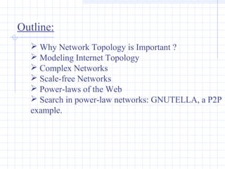
4. Modeling Internet Topology [1]:
 Graph representation
 Router-level modeling
- vertices are routers
-edges are one-hop IP connectivity
 Domain- (AS-) level model (high degree of abstraction)
- vertices are domains (ASes)
- edges are peering relationships
 Nodes can be assigned numbers rep. e.g. buffer
capacity
Edges migth have weights rep. e.g. – prop. delay,
bandwidth capacity.

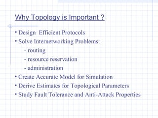
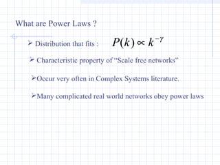
5. Modeling Internet Topology [1]:
transit domains
domains/autonomous systems
exchange point
border routers
peering
hosts/endsystems
routers
stub domains
access networks
lowly worm

6. Barabasi Albert Model (BA Model):
 Basis for most current topology generators
 Very simplistic model
Network evolves in size over time.
Preferential Connectivity
Probability that a newly added node will attach to node ‘i’
ki
Πi ) =
(k
Σ j
jk
 Many extensions.

7. Waxman Model:
 Router level model
 Nodes placed at random in 2D
space with dimension L
 Probability of edge (u,v):
a*e(-d / (bL) ), where d is
Euclidean distance (u,v), a and
b are constants
 Models locality
- no sense of backbone or hierarchy
- does not guarantee connected
network
- as #nodes ↑ the #links ↑
proportionally
u
d(u,v)
v

8. Transit-Stub Model:
Router level model
Transit domains
 placed in 2D space
 populated with routers
 connected to each other
Stub domains
 placed in 2D space
 populated with routers
 connected to transit domains
Models hierarchy
Edge count, guaranteed connectivity

9. Transit-Stub Model:
 No concept of a ‘host’ – all nodes are routers.
 Two level hierarchy
 First generate a number of transit domains,
then generate a set of stub networks.
 Given average edge-count, produce a
random graph, making sure that it is
connected.

10. Inet:
Generate degree sequence
Build spanning tree over nodes
with degree larger than 1, using
preferential connectivity
 randomly select node u not in
tree
 join u to existing node v with
probability d(v)/Σd(w)
Connect degree 1 nodes using
preferential connectivity
Add remaining edges using
preferential connectivity

11. BRITE:
Generate small backbone, with
nodes placed:
 randomly or
 concentrated (skewed)
Add nodes one at a time
(incremental growth)
New node has constant # of
edges connected using:
 preferential connectivity
and/or
 locality

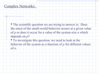
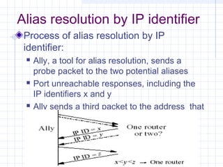
12. Complex Networks:
Two limiting-case topologies have been extensively considered in
the literature [4],[5].:
 regular network (lattice), the chosen topology of innumerable
physical models such as the Ising model or percolation.
 random graph, studied in mathematics and used both in
natural and social sciences. Properties studied in detail by Pal
Erdos.
 Most of Erdos’ work concentrated on the case in which the
number of vertices is kept constant but the total number of links
between vertices increases: the Erdös-Rényi result states that for
many important quantities there is a percolation-like transition
at a specific value of the average number of links per vertex.

13. Complex Networks:
 random networks are used in:
 Physics: in studies of dynamical problems, spin
models and thermodynamics, random walks, and
quantum chaos.
 Economics and social sciences: to model interacting
agents.

14. Complex Networks:
 In contrast to these two limiting topologies, empirical
evidence suggests that many biological, technological or
social networks appear to be somewhere in between these
extremes.
 many real networks seem to share with regular
networks the concept of neighborhood, which means that
if vertices i and j are neighbors then they will have many
common neighbors --- which is obviously not true for a
random network.
 On the other hand, studies on epidemics show that it
can take only a few ``steps'' on the network to reach a
given vertex from any other vertex. This is the foremost
property of random networks, which is not fulfilled by
regular networks.

15. Complex Networks:

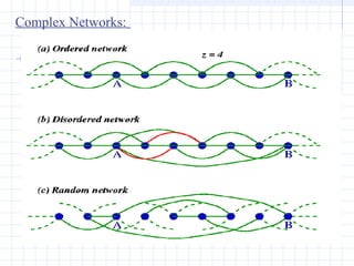
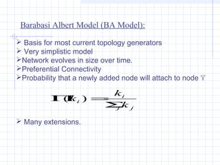
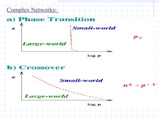
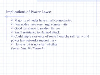
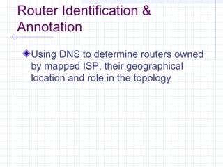
16. Complex Networks:
 The Watts-Strogatz model [5]. :
 To bridge the two limiting cases, Watts and Strogatz
[Nature 393, 440 (1998)] have introduced a new type of
network which is obtained by randomizing a fraction p of
the links of the regular network.
 Initial structure (p=0) is the one-dimensional regular
network where each vertex is connected to its z nearest
neighbors.
 For 0 < p < 1, we denote these networks disordered.
 for the case p=1, we have a completely random
network.

17. Complex Networks:
 Watts and Strogatz report that for a small value of the
parameter p, there is an onset of “small-world”
behavior.
 It is characterized by the fact that the distance between
any two vertices is of the order of that for a random
network and, at the same time, the concept of
neighborhood is preserved.
 The effect of a change in p is extremely nonlinear,
where a very small change in the connectivity of the
network leads to a dramatic change in the distance
between different pairs of vertices.

18. Complex Networks:
 The scientific question we are trying to answer is: Does
the onset of the small-world behavior occurs at a given value
of p or does it occur for a value of the system size n which
depends on p?
 To investigate this question, we need to look at the
behavior of the system as a function of p for different values
of n.

19. Complex Networks:

20. Complex Networks:
 The appearance of the small-world behavior is not a phasetransition but a crossover phenomena.
 The average distance l is:
l (n,p) ~ n* F ( n / n* )
where:
F(u << 1) ~ u, and F(u >> 1) ~ln u, and n* is a function of p.
 When the average number of rewired links, pnz/2, is much less
than one, the network should be in the large-world regime. On the
other hand, when pnz/2 >> 1, the network should be a small-world.

21. Scale-free networks:
 It was proposed by Barabási and Albert that real-world
networks in general are scale-free networks.
 Scale-free networks have a distribution of connectivities that
decays with a power-law tail.
 Scale-free networks emerge in the context of a growing
network in which new vertices connect preferentially to the
more highly connected vertices in the network. Scale free
networks are also small-world networks because (i) they have
clustering coefficients much larger than random networks, and
(ii) their diameter increases logarithmically with the number of
vertices n.

22. What are Power Laws ?
 Distribution that fits :
P(k ) ∝ k
−γ
 Characteristic property of “Scale free networks”
Occur very often in Complex Systems literature.
Many complicated real world networks obey power laws

23. Implications of Power Laws:
 Majority of nodes have small connectivity.
 Few nodes have very large connectivity.
 Good resistance to random failure.
 Small resistance to planned attack.
 Could imply existence of some hierarchy (all real world
power law networks support this).
 However, it is not clear whether
Power Law  Hierarchy

24. Origin of Power Law:
Power laws are an observed (empirical)
phenomenon.
The mechanisms that produce these can only be
guessed at (for now!)
Very typical in self organizing systems and chaotic
systems.

25. Scale-free networks:
 Scale-free networks:
(a) the neuronal network of the worm C. elegans.
(b) world-wide web.
(c) the network of citations of scientific papers.

26. Scale-free networks:
 broad-scale networks: or truncated scale-free networks,
characterized by a connectivity distribution that has a powerlaw regime followed by a sharp cut-off, like an exponential or
Gaussian decay of the tail.
 single-scale networks: characterized by a connectivity
distribution with a fast decaying tail, such as exponential or
Gaussian
Aging of the vertices: The vertex is still part of the network
and contributing to network statistics, but it no longer receives
links. The aging of the vertices thus limits the preferential
attachment preventing a scale-free distribution of connectivities.
 Cost of adding links to the vertices or the limited capacity of
a vertex: physical costs of adding links and limited capacity of a
vertex will limit the number of possible links attaching to a
given vertex.

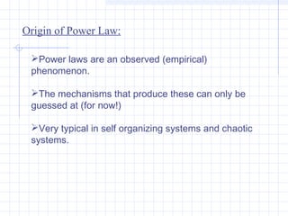
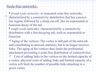
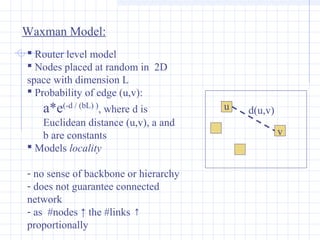
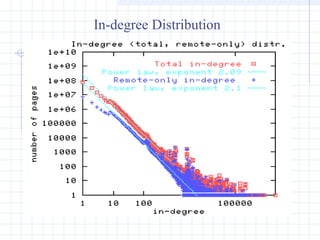
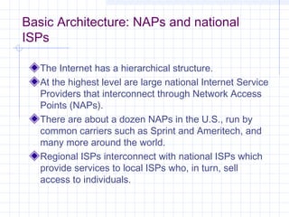
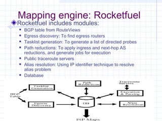
27. Power-laws of the Web [2].:
•How many links on a page (outdegree)?
• How many links to a page (indegree)?
•Probability that a random page has k other pages
pointing to it is ~k
-2.1
(Power law)
• Probability that a random page points to k other pages is
~k
-2.7
(Power law)

28. In-degree Distribution

29. Out-degree Distribution

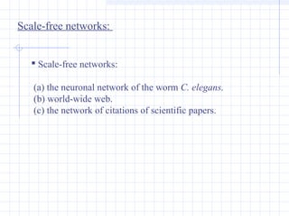
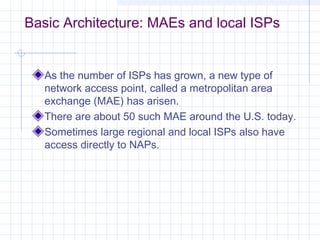
30. Search in power-law networks: GNUTELLA [3].
 Most of the P2P networks display a power-law
distribution in their node degree. This distribution
reflects the existence of a few nodes with very high
degree and many with low degree.
 In P2P networks, the name of the target file may be
known, but due to the network’s ad hoc nature, the node
holding the file may not be known until a real-time
search is performed.
 A simple strategy to locate files, implemented by
NAPSTER, is to use a central server that contains an
index of all the files every node is sharing as they join
the network.
 GNUTELLA and FREENET do not use a central
server.

31. Search in power-law networks: GNUTELLA [3].
 GNUTELLA is a peer-to-peer file-sharing system that treats
all client nodes as functionally equivalent and lacks a central
server that can store file location information. This is advantageous
because it presents no central point of failure.
 The obvious disadvantage is that the location of files is unknown.
When a user wants to download a file, he sends a query to
all the nodes within a neighborhood of size ttl, the time to
live assigned to the query. Every node passes on the query to
all of its neighbors and decrements the ttl by one. In this
way, all nodes within a given radius of the requesting node
will be queried for the file, and those who have matching
files will send back positive answers.

32. Search in power-law networks: GNUTELLA [3].
 This broadcast method will find the target file quickly,
given that it is located within a radius of ttl. However, broadcasting
is extremely costly in terms of bandwidth.
 Such a search strategy does not scale well. As query traffic
increases linearly with the size of GNUTELLA graph, nodes
become overloaded.

33. Search in power-law networks: GNUTELLA [3].
 Typically, a GNUTELLA client wishing to join the network
must find the IP address of an initial node to connect to.
Currently, ad hoc lists of ‘‘good’’ GNUTELLA clients exist.
 It is reasonable to suppose that this ad hoc method of
growth would bias new nodes to connect preferentially to
nodes that are already fairly well connected, since these
nodes are more likely to be ‘‘well known.’’
 Based on models of graph growth where the ‘‘rich get richer,’’
the power-law connectivity of ad hoc peer-to-peer networks may
be a fairly general topological feature.

34. Search in power-law networks: GNUTELLA [3].
 By passing the query to every single node in the network,
the GNUTELLA algorithm fails to take advantage of the
connectivity distribution [3].
 To take advantage of the power-law distribution, we can modify
each node to keep lists of files stored in first and second neighbor.
 Instead of passing the query to every node, now we can pass it
only to the nodes with highest connectivity.
 High degree nodes are presumably high bandwidth node that can
handle the query traffic.

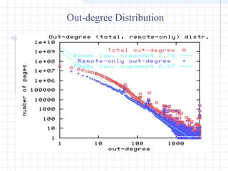
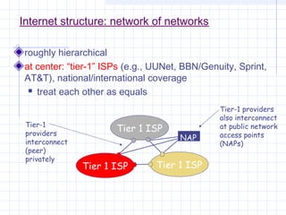
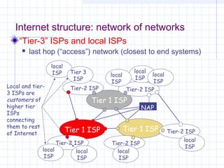
35. Outline:
Internet Structure
&Organization
 Internet Hierarchical Structure
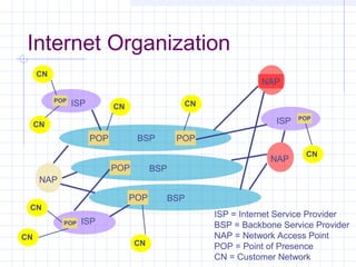
 ISPs, interconnection and organization [ref. 7].
 POP Architecture and Load Balancing
 ISP Architecture [ref. 7]. in detail
 Topology Mapping Tool: Rocketfuel[ref. 8]
 Discussion
ELEG 667-013 Spring 2003

36. Basic Internet Architecture

37. Basic Architecture: NAPs and national
ISPs
The Internet has a hierarchical structure.
At the highest level are large national Internet Service
Providers that interconnect through Network Access
Points (NAPs).
There are about a dozen NAPs in the U.S., run by
common carriers such as Sprint and Ameritech, and
many more around the world.
Regional ISPs interconnect with national ISPs which
provide services to local ISPs who, in turn, sell
access to individuals.

38. Basic Architecture: MAEs and local ISPs
As the number of ISPs has grown, a new type of
network access point, called a metropolitan area
exchange (MAE) has arisen.
There are about 50 such MAE around the U.S. today.
Sometimes large regional and local ISPs also have
access directly to NAPs.

39. Internet Packet Exchange Charges
ISP at the same level usually do not charge each
other for exchanging messages.
This is called peering.
Higher level ISPs, however, charge lower level ones
(national ISPs charge regional ISPs which in turn
charge local ISPs) for carrying Internet traffic.
Local ISPs, of course, charge individuals and
corporate users for access.

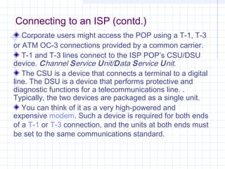
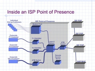
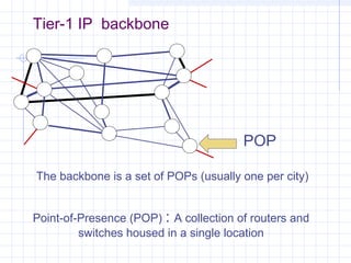
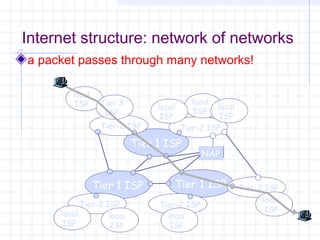
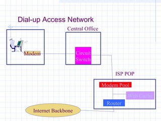
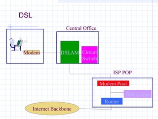
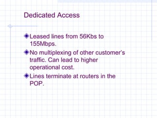
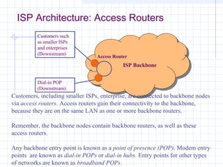
40. Connecting to an ISP
ISPs provide access to the Internet through a Point of
Presence (POP).
Individual users access the POP through a dial-up
line using the PPP protocol.
The call connects the user to the ISP’s modem pool,
after which a remote access server (RAS) checks the
userid and password.
Once logged in, the user can send TCP/IP/[PPP]
packets over the telephone line which are then sent
out over the Internet through the ISP’s POP.

41. Connecting to an ISP (contd.)
Corporate users might access the POP using a T-1, T-3
or ATM OC-3 connections provided by a common carrier.
T-1 and T-3 lines connect to the ISP POP’s CSU/DSU
device. Channel Service Unit/Data Service Unit.
The CSU is a device that connects a terminal to a digital
line. The DSU is a device that performs protective and
diagnostic functions for a telecommunications line. .
Typically, the two devices are packaged as a single unit.
You can think of it as a very high-powered and
expensive modem. Such a device is required for both ends
of a T-1 or T-3 connection, and the units at both ends must
be set to the same communications standard.

42. Inside an ISP Point of Presence
Individual
Dial-up Customers
ISP POP
ISP Point-of Presence
Modem Pool
Corporate
T1 Customer
Corporate
T3 Customer
Corporate
OC-3 Customer
ISP POP
T1 CSU/DSU
Layer-2
Switch
ATM
Switch
ISP POP
T3 CSU/DSU
ATM Switch
Remote
Access
Server
NAP/MAE

43. Internet Organization
CN
NAP
POP
ISP
CN
CN
ISP
CN
BSP
POP
POP
POP
POP
BSP
NAP
CN
NAP
POP
CN
POP
CN
ISP
CN
BSP
ISP = Internet Service Provider
BSP = Backbone Service Provider
NAP = Network Access Point
POP = Point of Presence
CN = Customer Network

44. Customer Network
Clients
LAN
Servers
Ethernet
10 Mb/s
Router
WAN
T1 Link
1.54 Mb/s

45. NAP Architecture
ISP
ISP
ISP
Backbone
Operator
Routers
Route
Server
High-Speed LAN (FDDI, ATM, GigE)
Routers
Backbone
Operator
ISP
Backbone
NAP
Operator

46. Internet structure: network of networks
roughly hierarchical
at center: “tier-1” ISPs (e.g., UUNet, BBN/Genuity, Sprint,
AT&T), national/international coverage
 treat each other as equals
Tier-1
providers
interconnect
(peer)
privately
Tier 1 ISP
Tier 1 ISP
NAP
Tier 1 ISP
Tier-1 providers
also interconnect
at public network
access points
(NAPs)

47. Tier-1 ISP: e.g., Sprint
Sprint US backbone network

48. Tier-1 IP backbone
POP
The backbone is a set of POPs (usually one per city)
Point-of-Presence (POP) : A collection of routers and
switches housed in a single location

49. Internet structure: network of networks
“Tier-2” ISPs: smaller (often regional) ISPs

Connect to one or more tier-1 ISPs, possibly other tier-2 ISPs
Tier-2 ISP pays
tier-1 ISP for
connectivity to
rest of Internet
 tier-2 ISP is
customer of
tier-1 provider
Tier-2 ISP
Tier-2 ISP
Tier 1 ISP
Tier 1 ISP
Tier-2 ISP
NAP
Tier 1 ISP
Tier-2 ISP
Tier-2 ISPs
also peer
privately with
each other,
interconnect
at NAP
Tier-2 ISP

50. Internet structure: network of networks
“Tier-3” ISPs and local ISPs

last hop (“access”) network (closest to end systems)
local
ISP
Local and tier3 ISPs are
customers of
higher tier
ISPs
connecting
them to rest
of Internet
Tier 3
ISP
Tier-2 ISP
local
ISP
local
ISP
local
ISP
Tier-2 ISP
Tier 1 ISP
Tier 1 ISP
Tier-2 ISP
local
local
ISP
ISP
NAP
Tier 1 ISP
Tier-2 ISP
local
ISP
Tier-2 ISP
local
ISP

51. Internet structure: network of networks
a packet passes through many networks!
local
ISP
Tier 3
ISP
Tier-2 ISP
local
ISP
local
ISP
local
ISP
Tier-2 ISP
Tier 1 ISP
Tier 1 ISP
Tier-2 ISP
local
local
ISP
ISP
NAP
Tier 1 ISP
Tier-2 ISP
local
ISP
Tier-2 ISP
local
ISP

52. Architecture of a POP
Backbone links
Backbone
Router
Backbone
Router
Peering
Access
Router
Access
Router
Access
Router
Access
Router
ISPs
Corporate
networks
Web Servers
Dial-up

53. ISP Architecture
Access Network Architecture





Dial-up
ISDN
DSL
Dedicated Leased lines
Frame Relay Service

54. Dial-up Access Network
Central Office
Modem
Circuit
Switch
ISP POP
Modem Pool
Web Cache
Router
Internet Backbone

55. ISDN
ISDN service access links
terminate at the ISP POP
Digital signal. Due to signal
strength limitations, ISDN
subscribers must be within 18000
feet of the CO
At the customers end, an ISDN
adapter card is required.

56. DSL
Central Office
Modem
DSLAM Circuit
Switch
ISP POP
Modem Pool
Web Cache
Router
Internet Backbone

57. DSL Access
DSL typically provisioned at 1.5Mbps
from ISP to customer and at 128kbs in
the reverse direction.
DSL Access Multiplexer (DSLAM) at
CO terminates DSL signals from
hundreds of customers.
The IP data is multiplexed into a single
ATM connection by DSLAM and
forwarded to the ISP POP

58. Dedicated Access
Leased lines from 56Kbs to
155Mbps.
No multiplexing of other customer’s
traffic. Can lead to higher
operational cost.
Lines terminate at routers in the
POP.

59. Frame Relay Service
Network resembles a star topology, with
one leg of the star connected to ISP and
other legs connected to different
customers.
Router
Frame Relay
Network
Router
Router
ISP
Router

60. ISP Architecture: The Backbone
Backbone router
ISP Backbone
The backbone of a large ISP is typically a WAN spread out across a large
geographic area.
Backbone routers connect the individual links composing the backbone .

61. ISP Architecture: Backbone Nodes
Backbone Node
Backbone Node
ISP Backbone
For reasons of robustness and load management, multiple backbone routers
can be located in the same geographic location and connected via a LAN.
We consider all of the backbone routers and the connecting LAN to be
a backbone node.
These backbone nodes, whether they contain one or more routers, will serve
as the points of connection from the outside world to the backbone.

62. ISP Architecture: Access Routers
Customers such
as smaller ISPs
and enterprises
(Downstream)
Access Router
ISP Backbone
Dial-in POP
(Downstream)
Customers, including smaller ISPs, enterprise, are connected to backbone nodes
via access routers. Access routers gain their connectivity to the backbone,
because they are on the same LAN as one or more backbone routers.
Remember, the backbone nodes contain backbone routers, as well as these
access routers.
Any backbone entry point is known as a point of presence (POP). Modem entry
points are known as dial-in POPs or dial-in hubs. Entry points for other types
of networks are known as broadband POPs.

63. ISP Architecture: In Practice
Broadband POP
Access Router
ISP Backbone
Large dial-in POP
(Downstream)
Backbone Router
In practice, only the largest customers connect directly to access routers. Other
customers are aggregated at broadband points of presence (broadband POPs).
These are basically LANs. The customers connect to routers on these LANs, and
then these LANs connect to the access nodes
Additionally, some very large dial-in POPs do connect directly to backbone routers.
These typically service very large corporate offices.

64. ISP Architecture: Gateways
Upstream ISP
ISP Backbone
Peer ISP
Gateway Router
Gateway routers, which are also connected via LANs to backbone routers,
connect ISPs to each other. The router is known as a gateway router, if it connects
a peer or upstream ISP.
Downstream ISPs generally connect via an access router, or directly to a backbone
Router.
So, a gateway router leads to a peer or upstream provider, whereas an access router leads to
a downstream network.

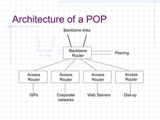
65. Measuring ISP Topologies with Rocketfuel[8]:
 Rocketfule – internet topology mapping engine
 The goal is to obtain realistic, router-level maps of ISP networks.
 Important influence on:
- The dynamics of routing protocols
- The scalability of multicast
- The efficacy of proposals for denial-of-service tracing and
response
- Other aspects of protocol performance (Internet path
selection)
 Real topologies are not publicly available
- Confidential

66. Mapping techniques
Three categories of mapping
techniques:

Selecting Measurements
 Directed probing
 Path reduction

Alias Resolution
 IP identifier

Router identification and Annotation

67. Selecting Measurements
Directed probing

To employ BGP tables to identify relevant
traceroutes and prune the remainder
Path reduction

To identify redundant traceroutes
 Only one traceroutes needs to be taken when
two traceroutes enter and leave the ISP
network at the same point

68. Alias resolution
Mercator method

Sending traceroute-like probe(to a highnumbered UDP port but with a TTL of 255)
directly to the potentially aliased IP
address
 Requirement: routers need to be configured to
send the “UDP port unreachable” response
with the address of the outgoing interface as
the source address: Two aliases should
respond with the same source

69. Alias method
Proposed methods by Spring etc.


Mercator’s IP address-based method
Comparing IP identifier field of the
responses

70. IP identifier hints
IP identifier helps to identify a packet for
reassembly after fragmentation
IP identifier is commonly implemented
using a counter that is incremented
after sending a packet

71. Alias resolution by IP identifier
Process of alias resolution by IP
identifier:



Ally, a tool for alias resolution, sends a
probe packet to the two potential aliases
Port unreachable responses, including the
IP identifiers x and y
Ally sends a third packet to the address that
responded first

72. Router Identification &
Annotation
Using DNS to determine routers owned
by mapped ISP, their geographical
location and role in the topology

73. Mapping engine: Rocketfuel
Rocketfuel includes modules:







BGP table from RouteViews
Egress discovery: To find egress routers
Tasklist generation: To generate a list of directed probes
Path reductions: To apply ingress and next-hop AS
reductions, and generate jobs for execution
Public traceroute servers
Alias resolution: Using IP identifier technique to resolve
alias problem
Database

74. References:
[1] Kenneth Calvert, Matthew Doar, Ellen Zegura, “Modeling Internet
Topology”.
[2]. Michalis Faloudsos, Petros Faloudsos, Christos Faloudsos, “On
Power-law Relationships of the Internet Topology”
[3]. Lada A. Adamic,1, Rajan M. Lukose,1, Amit R. Puniyani,2, and
Bernardo A. Huberman1,” Search in power-law networks”.
[4]. L. A. N. Amaral, A. Scala, M. Barthélémy, & H. E. Stanley, 1997,
“Classes of small-world networks.”
http://polymer.bu.edu/~amaral/Content_network.html
[5]. Ellen Zegura, Kenneth Calvert, “How to model an Internetwork”
[6]. Stefan Bornholdt, Holger Ebel, “World Wide Web scaling
exponent from Simon’s 1955 model”
[7]. S. Halabi and D. McPherson, Internet Routing Architectures, 2nd
ed., Cisco Press, Indianapolis, 2000.
[8]. Neil Spring Ratul Mahajan David Wetherall, Measuring ISP
Topologies with Rocketfuel