Download to read offline


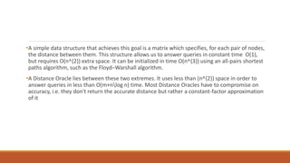
![Fast Mincut algorithm
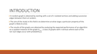
Input: A multigraph G=(V,E)
Output: A cut C
1.Let n:=|V|
2.If n<=6 then compute mincut of G directly else
◦ t:=[1+n/√2]
◦ Call contraction(t) twice (independently) to produce to graphs H1 and H2
◦ Let C1=Fastmincut(H1) and C2=Fastmincut(H2)
◦ C=min{C1,C2}](https://image.slidesharecdn.com/optimisationrandomgraphpresentation-170505122539/85/Optimisation-random-graph-presentation-19-320.jpg)
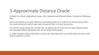
![Complexity
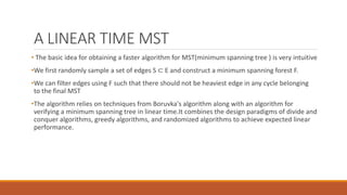
•The probability that a specific mincut C survives at the end of Contraction(t) is at least
[t(t-1)/n(n-1)]
• Therefore contraction(2) produces a mincut with probability 𝛺 1/𝑛2 .
•For Fast mincut algorithm it follows the following recurrence
•T(n)=2T([1+n/ 2]) + 𝑂(𝑛2
).
•Solving this recurrence we get T(n)=O(nlogn).](https://image.slidesharecdn.com/optimisationrandomgraphpresentation-170505122539/85/Optimisation-random-graph-presentation-20-320.jpg)


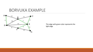
The document discusses randomized graph algorithms and techniques for analyzing them. It describes a linear time algorithm for finding minimum spanning trees (MST) that samples edges and uses Boruvka's algorithm and edge filtering. It also discusses Karger's algorithm for approximating the global minimum cut in near-linear time using edge contractions. Finally, it presents an approach for 3-approximate distance oracles that preprocesses a graph to build a data structure for answering approximate shortest path queries in constant time using landmark vertices and storing local and global distance information.


![Reduction of multiple subsystem [compatibility mode]](https://cdn.slidesharecdn.com/ss_thumbnails/reductionofmultiplesubsystemcompatibilitymode-110418075355-phpapp01-thumbnail.jpg?width=640&height=640&fit=bounds)


![Human Reproduction [ Reproductive System ] Notes @irfanullah_mehar Irfanullah...](https://cdn.slidesharecdn.com/ss_thumbnails/humanreproductionreproductivesystemnotesirfanullahmeharirfanullahmeharjanantantra-260111172350-56e85778-thumbnail.jpg?width=640&height=640&fit=bounds)


