Download as PDF, PPTX


![Bucket Sort
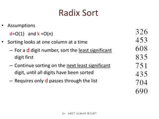
• Assumption:
– the input is generated by a random process that distributes elements
uniformly over [0, 1]
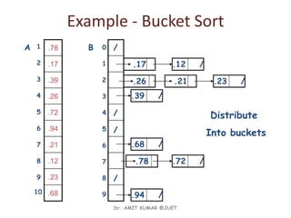
• Idea:
– Divide [(0, 1) into k equal-sized buckets (k=Θ(n))]
– Distribute the n input values into the buckets
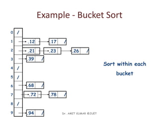
– Sort each bucket (e.g., using quicksort)
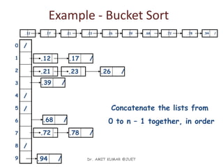
– Go through the buckets in order, listing elements in each one
• Input: A[1 . . n], where 0 ≤ A[i] < 1 for all i
• Output: elements A[i] sorted
Dr. AMIT KUMAR @JUET](https://image.slidesharecdn.com/linearsort-180514053152/85/Linear-sort-6-320.jpg)
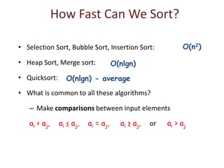
![Bucket sort algorithm
Algorithm BucketSort( S )
( values in S are between 0 and m-1 )
for j 0 to m-1 do // initialize m buckets
b[j] 0
for i 0 to n-1 do // place elements in their
b[S[i]] b[S[i]] + 1 // appropriate buckets
i 0
for j 0 to m-1 do // place elements in buckets
for r 1 to b[j] do // back in S
S[i] j
i i + 1
Dr. AMIT KUMAR @JUET](https://image.slidesharecdn.com/linearsort-180514053152/85/Linear-sort-11-320.jpg)

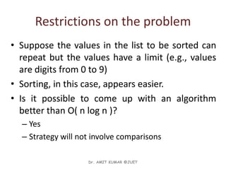
![Analysis of Bucket Sort
Alg.: BUCKET-SORT(A, n)
for i ← 1 to n
do insert A[i] into list B[nA[i]]
for i ← 0 to k - 1
do sort list B[i] with quicksort sort
concatenate lists B[0], B[1], . . . , B[n -1]
together in order
return the concatenated lists
O(n)
k O(n/k log(n/k))
=O(nlog(n/k)
O(k)
O(n) (if k=Θ(n))
Dr. AMIT KUMAR @JUET](https://image.slidesharecdn.com/linearsort-180514053152/85/Linear-sort-13-320.jpg)

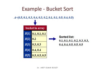
![Counting Sort
• Assumptions:
– n integers which are in the range [0 ... r]
– r is in the order of n, that is, r=O(n)
• Idea:
– For each element x, find the number of elements x
– Place x into its correct position in the output array
output array
Dr. AMIT KUMAR @JUET](https://image.slidesharecdn.com/linearsort-180514053152/85/Linear-sort-26-320.jpg)
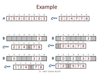
![Algorithm
• Start from the last element of A
• Place A[i] at its correct place in the output array
• Decrease C[A[i]] by one
30320352
1 2 3 4 5 6 7 8
A
77422
1 2 3 4 5
Cnew 8
0
Dr. AMIT KUMAR @JUET](https://image.slidesharecdn.com/linearsort-180514053152/85/Linear-sort-29-320.jpg)
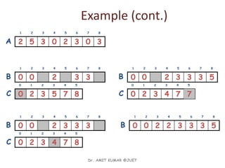
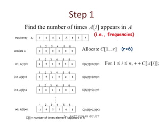
![COUNTING-SORT ALGO
Alg.: COUNTING-SORT(A, B, n, k)
1. for i ← 0 to r
2. do C[ i ] ← 0
3. for j ← 1 to n
4. do C[A[ j ]] ← C[A[ j ]] + 1
5. C[i] contains the number of elements equal to i
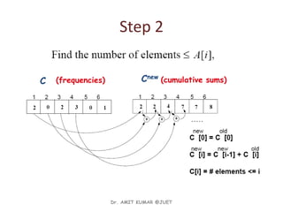
6. for i ← 1 to r
7. do C[ i ] ← C[ i ] + C[i -1]
8. C[i] contains the number of elements ≤ i
9. for j ← n downto 1
10. do B[C[A[ j ]]] ← A[ j ]
11. C[A[ j ]] ← C[A[ j ]] - 1
1 n
0 k
A
C
1 n
B
j](https://image.slidesharecdn.com/linearsort-180514053152/85/Linear-sort-32-320.jpg)
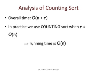
![Analysis of Counting Sort
Alg.: COUNTING-SORT(A, B, n, k)
1. for i ← 0 to r
2. do C[ i ] ← 0
3. for j ← 1 to n
4. do C[A[ j ]] ← C[A[ j ]] + 1
5. C[i] contains the number of elements equal to i
6. for i ← 1 to r
7. do C[ i ] ← C[ i ] + C[i -1]
8. C[i] contains the number of elements ≤ i
9. for j ← n downto 1
10. do B[C[A[ j ]]] ← A[ j ]
11. C[A[ j ]] ← C[A[ j ]] - 1
O(r)
O(n)
O(r)
O(n)
Overall time: O(n + r)](https://image.slidesharecdn.com/linearsort-180514053152/85/Linear-sort-33-320.jpg)


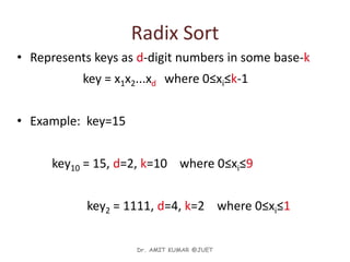
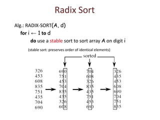
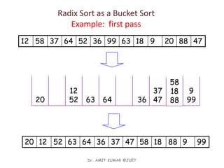
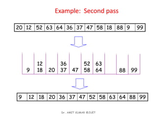
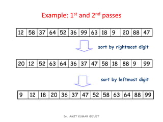
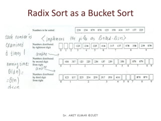
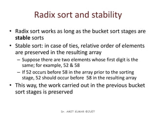
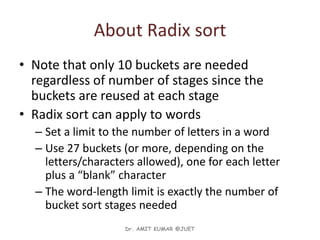
Linear sorting algorithms like counting sort, bucket sort, and radix sort can sort arrays of numbers in linear O(n) time by exploiting properties of the data. Counting sort works for integers within a range [0,r] by counting the frequency of each number and using the frequencies to place numbers in the correct output positions. Bucket sort places numbers uniformly distributed between 0 and 1 into buckets and sorts the buckets. Radix sort treats multi-digit numbers as strings by sorting based on individual digit positions from least to most significant.